


Ordinary differential equations (and initial value problems)#
In mathematics, an ordinary differential equation (ODE) is a differential equation (DE) dependent on only a single independent variable. As with other DE, its unknown(s) consists of one (or more) function(s) and involves the derivatives of those functions The term “ordinary” is used in contrast with partial differential equations which may be with respect to more than one independent variable.(see https://en.wikipedia.org/wiki/Ordinary_differential_equation?useskin=vector)
An initial value problem, IVP, is a a problem specified by an ordinary differential equation and its initial conditions.
You have been already solving a differential equation: The second Newton law
Can be seen as a first order differential equation (when talking about \(v\)) or as a second order differential equation (regarding \(x\)).
For instance, a projectile must follow a parabolic path, but that is because the parabolic path is the solution for the corresponding differential equation.

The following geogebra applet shows the effect of fixing the initial condition: https://www.geogebra.org/m/pepN3KbH
In this chapter we will focus on solving, numerically, Ordinary differential equations. Later we will learn some basic methods for Partial differential equations. For a nice introduction to both of them, please watch:
A numerical solution for and IVP corresponds to finding an algorithm that allows you to move from time \(t\) to time \(t+\delta t\), given a time discretization. It is assumed that the general problem is represented as
where \(y\) represents the state of the system. All linear differential equations of any order can be cast to this form by introducing auxiliary derivatives, so the problem becomes vectorial, but its form remains
So the key question is how to go numerically from \(\vec y(t)\) to \(\vec y(t+\delta t)\). There are several algorithms, with both advantages and disadvantages (in sinplicity, precision, stability, etc), to do so. Here we will see Euler algorithm which is the most straight forward (but lacks precision and stability), and later one of the most common, the Runge-Kutta. After that, specific algorithms for second order equations will be discussed (like Leap-Frog and Verlet), and, finally some numerical libraries will be shown.
Why Do We Need Numerical Methods?#
Many of the equations that appear in introductory physics courses admit elegant analytical solutions. Examples include projectile motion without air resistance, the simple harmonic oscillator, and exponential radioactive decay.
However, most realistic physical systems are governed by differential equations that cannot be solved exactly. In these cases, numerical methods are not merely convenient—they are essential.
Some important examples are:
The gravitational interaction of three or more bodies (the N-body problem).
The motion of a double pendulum.
Turbulent fluid flows.
Molecular dynamics simulations involving thousands of interacting particles.
Weather and climate models.
Chaotic systems such as the Lorenz equations.
In all these cases, the governing equations are known, but no closed-form analytical solution exists. Instead, we compute approximate solutions by integrating the equations step by step on a computer.
The goal of this chapter is to understand how such numerical integration methods work, beginning with the simplest approach: Euler’s method.
Example: The Three-Body Problem#
Consider three masses interacting through Newtonian gravity. For each body,
Unlike the two-body problem, which leads to the familiar Keplerian orbits, no general analytical solution is known for three interacting bodies.
Even though the equations are straightforward to write down, predicting the motion requires numerical integration.
You can see and interactive three-body problem simulation at Trisolar chaos
import IPython
IPython.display.HTML('assets/ode_method_comparison.html')
First order algorithm: The Euler algorithm#
The Euler method is based on the forward derivative:
Here, \(h = \delta t\). Since we are looking for \(f(t + \delta t)\), and we actually know the derivatives (they are given by the differential equation we want to solve), then
Where \(\vec f(t, \vec y) = d\vec y/dt\) is just the function returning the derivatives. As you can see , basically the Euler method is performing a linear extrapolation.
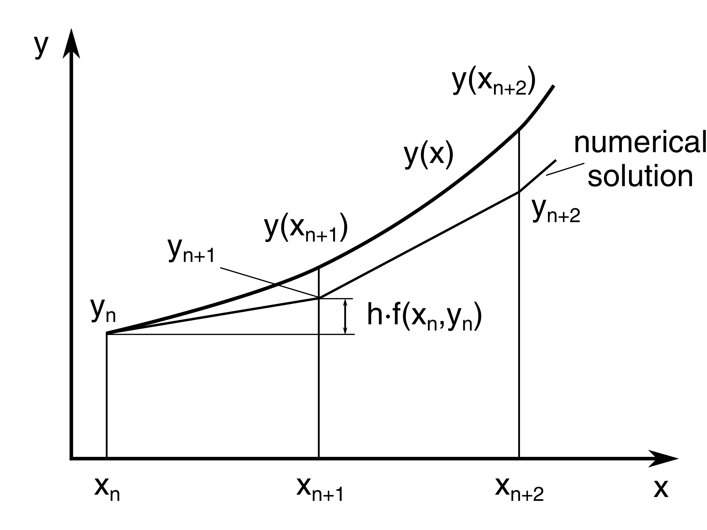
Although easy to implement, it lacks stability, and its low order (locally \(O(\delta t^2)\), globally \(O(N\delta t^2) = O(\delta t)\)) implies a very small \(\delta t\), so many steps to solve the IVP on a given time interval.
Second order algorithm : The Heun method#
https://en.wikipedia.org/wiki/Heun’s_method?useskin=vector

The Heun method, also known as the improved Euler method, mid-point method, or second order Runge-Kuta mehtod, is an improvement over the initial Euler method.
Here, you need to compute intermediate values to estimate better the final value at each step:
Fourth order algorithm: Runge-Kutta algorithm RK4#
Here, we will study the typical Runge-Kutta method of order 4, for N coupled linear differential equations. This is much better than simple Euler. The price to pay is to evaluate the derivatives four times per time step.

For the RK4 algorithm , we can compute the evolution as
with the \(\vec k_i\) functions evaluating the derivatives at different stages
The total global order is \(O(\delta t^4)\).
Implementation discussion: introduction to c++ templates#
To implement any of the following approaches, please think about the requirements for the function to do that, before writing any code. Like:
It needs to receive the initial and final times, plus the time step.
Given that all methods need the current state, it should be given as an argument (as a reference to avoid creating costly copies when N is large)
It should receive the derivatives function, to be able to compute the derivatives.
EXTRA: To be able write the data in any chosen way, it might get a function to write the data, and that function must get the time, the state and the derivatives.
Do you think something else is needed?
Therefore, something like the following is needed:
template <class deriv_t, class system_t, class printer_t>
void integrate(deriv_t fderiv, system_t & s, double tinit, double tend, double dt, printer_t && writer);
where:
state_trepresents the system state, likestd::valarray<double>orstd::vector<double>.deriv_trepresents the function type that compute the derivatives, which in turn should be likevoid fderiv(const system_t & s, system_t & dsdt, double t). Notice the const and non-const on the arguments.printer_trepresents a function type used to print, likevoid printer(const system_t & s, double t)or a lambda. To accept any object, we use a forwarinding reference&&which adapts to any type.
When a function can work with several generic types as shown, one can use templates. But we can also use using fptr = std::fuction.... To learn more, we will use templates! (this makes us put the implementation in the header files).
To represent the system state \(s\) we can use std::valarray which will avoid using many for loops.
Example: implementing the Euler method for a one dimensional problem#
Here we will solve the following one dimensional differential equation :
where \(r\) is a parameter. This equation is called the “logistic equation” and used in the population dynamics field (https://en.wikipedia.org/wiki/Logistic_function?useskin=vector#Logistic_differential_equation).

This is also related to chaos through the logistic map: https://en.wikipedia.org/wiki/Logistic_map?useskin=vector
For our solver, we have the following template implementation: Notice that the solver knows nothing about your functions for writing, the system data struct used and so on.
// ivp_solver.h
#include <iostream>
#include <valarray>
#include <functional>


// function template to work with "any" type
template <class deriv_t, class system_t, class printer_t>
void integrate_euler(deriv_t fderiv, system_t & s, double tinit, double tend, double dt, printer_t writer)
{
    // vector to store derivs
    system_t dsdt(s.size());

    // time loop
    for(double t = tinit; t <= tend; t = t + dt) { // NOTE: Last time step not necessarily tf
        // compute derivs
        fderiv(s, dsdt, t);

        // compute new state. NOTE: Not using components, assuming valarray or similar
       // TODO: Complete the code here

        // write new state
        writer(s, t);
      }
}
and the main file would be
Warning
Use of std::valarray We use std::valarray for its convenient mathematical syntax and lack of external dependencies. For high-performance or large-scale simulations, physicists typically migrate to dedicated linear algebra libraries like Eigen or Armadillo.
#include <iostream>
#include <valarray>
#include <cmath>
#include "ivp_solver.h"

const double R = 3.5;

typedef std::valarray<double> state_t; // alias for state type

void initial_conditions(state_t & y);
void print(const state_t & y, double time);
void fderiv(const state_t & y, state_t & dydt, double t);

int main(int argc, char **argv)
{
    int N = 1;
    state_t y(N);
    initial_conditions(y);
    integrate_euler(fderiv, y, 0.0, 10.0, 0.01, print);
    return 0;
}

void initial_conditions(state_t & y)
{
  y[0] = 0.5;
}

void print(const state_t & y, double time)
{
  std::cout << time << "\t" << y[0] << std::endl;
}

void fderiv(const state_t & y, state_t & dydt, double t)
{
    // TODO: Complete the code here

}
Exercise 18
Complete the code and solve the system for several \(r\) values.
The Lorenz model and attractor#
The Lorenz model for climate represents a coupled system of one-dimensional differential equations that is used to study the climate and also gave the first evidence on sensitivy to initial conditions and the onset of chaos. Its solutions attractor is very famous:

It is represented as the following set of coupled equations:
As you can see, we have three independet variables, and three parameters.
Exercise : Solve using the Euler method#
Adapt the previous main code to solve the Lorenz system. Select some parameter values and plot two solutions that start very close. Use \(\sigma=10, \rho=28, \beta=8/3\)
Exercise: Heun method#
Implement the Heun method (integrate_heun) and solve again. DO you find any precision difference with the Euler method?
Solving a second order differential equation#
A typical second order example is the famous harmonic oscillator, described by
which can be transformed into a system of 2 differential equations using the velocity, \(v = dx/dt\), as \(\vec y = (y_0, y_1) = (x, dx/dt) = (x, v)\),
Therefore, in this case the state vector will have 2 components: The first one for the position, the second one for the velocity.
In this particular case we will need a parameter, \(\omega\). In general, remember that if you need parameters (mass, frequency, spring constant) you either use lambda functions or functors to model the system derivatives and keep the derivative interface uniform. For instance, our derivative funtcion could be a lambda like
double W = ...;
// actual derivatives: this is the system model
auto fderiv = [W](const state_t & y, state_t & dydt, double t){
    dydt[0] = y[1];
    dydt[1] = -W*W*y[0];
};
Exercises#
Solve the simple harmonic oscillator: energy conservation#
Solve the system, for \(\omega = 1.234\) rad/s. Choose an appropriate time interval so you have at least for full oscillations. Again, plot the theoretical and numerical solutions for \(\delta t = 0.1, 0.2, 0.5, 1.0\). Furthermore, plot the mechanical energy as function of time, and also plot the phase space \(v\) versus \(x\).
Solve the simple harmonic oscillator: energy conservation with Heun#
Do the same but with the Heun method
Phase space#
Plot \(v_x\) versus \(x\). Can you predict the expected trajectory? do it for both euler and heun.
Streamlines#
Use matplotlib streamlines function to plot the phase space for many initial conditions. Do it for both the linear and nonlinear pendulum.
Runge-Kutta algorithm of fourth order: Implementation#
Unfortunately, the Euler method is not stable, and its precision is far from ideal. We can improve its order by using methods that or order 3, 4 and so on. Here, we will study the typical Runge-Kutta method of order 4, for N coupled linear differential equations. This is much better than simple Euler. The price to pay is to evaluate the derivatives four times per time step.
According to the Runge-Kutta algorithm, we will need to go step by step
computing k1, k2, ... and then update the state. We will compute the
derivatives four times per time step, but the gain in precision will be huge, compared to the Euler.
To implement this, we just add a new function to our integrator.cpp file, adding the
following implementation
template <class deriv_t, class system_t, class printer_t>
void integrate_rk4(deriv_t fderiv, system_t & s, double tinit, double tend, double dt, printer_t writer)
{
    // vector to store derivs
    system_t k1, k2, k3, k4, aux;
    const int N = s.size();
    k1.resize(N); k2.resize(N); k3.resize(N); k4.resize(N); aux.resize(N);

    // time loop
    for(double t = tinit; t <= tend; t = t + dt) { // NOTE: Last time step not necessarily tf
        // k1 -> (t, y)
        fderiv(s, k1, t);
        // k2 -> t+h/2, y+h*k1/2
        aux = s + k1*dt/2;
        fderiv(aux, k2, t + dt/2);
        // TODO


        // use all k
        s = s + dt*(k1 + 2*k2 + 2*k3 + k4)/6.0;
        // call writer
        writer(s, t);
    }
}
Exercise#
Implement the rk4 and use it to check the energy conservation for the harmonic oscillator. Is it better than Euler?
Exercises#
Compare the results for the same system and same \(\Delta t\) using both Euler and rk4. Does rk4 conserves the mechanical energy better?
Make the oscillator non-linear, with a force of the form \(F(x) = -kx^\lambda\), with \(\lambda\) even. How is the system behaviour as you change \(\lambda\)?
Add some damping to the linear oscillator, with the form \(f_{damp} = -mbv\), where \(m\) is the mass and \(b\) the damping constant. Plot the phase space. Comment about the solution.
Solve many dynamical system that you can find in any numerical programming book.
Implement the leap-frog method: https://en.wikipedia.org/wiki/Leapfrog_integration?useskin=vector. Notice that you need a spetial treatment to start the algorithm.
Implement the Verlet method: https://en.wikipedia.org/wiki/Verlet_integration?useskin=vector . Notice that you need a spetial treatment to start the algorithm.
Using a library : odeint#
You could also use more elaborate libraries tailored to this kind of problems. In this section we will use odeint, https://headmyshoulder.github.io/odeint-v2/examples.html . Install it if you don’t have it. In the computer room it is already installed. The interface is pretty similar to what we have been doing, but it includes much more advanced algorithms (this is analogous to using scipy). Use the following example as a base code
#include <iostream>
#include <vector>
#include <cmath>
#include <cstdlib>
#include <boost/numeric/odeint.hpp>

typedef std::vector<double> state_t; // alias for state type

void initial_conditions(state_t & y);
void print(const state_t & y, double time);
void fderiv(const state_t & y, state_t & dydt, double t);

int main(int argc, char **argv)
{
  if (argc != 5) {
    std::cerr << "ERROR. Usage:\n" << argv[0] << " T0 TF DT W" << std::endl;
    std::exit(1);
  }
  const double T0 = std::atof(argv[1]);
  const double TF = std::atof(argv[2]);
  const double DT = std::atof(argv[3]);
  const double W  = std::atof(argv[4]);
  const int N = 2;

  auto fderiv = [W](const state_t & y, state_t & dydt, double t){
    dydt[0] = y[1];
    dydt[1] = -W*W*y[0];
  };

  state_t y(N);
  initial_conditions(y);
  boost::numeric::odeint::integrate(fderiv, y, T0, TF, DT, print);

  return 0;
}

void initial_conditions(state_t & y)
{
  y[0] = 0.9876;
  y[1] = 0.0;
}

void print(const state_t & y, double time)
{
  std::cout << time << "\t" << y[0] << "\t" << y[1] << std::endl;
}
Exercises#
Again, compare the errors among euler, rk4 and odeint.
Use a functor to encapsulate the global parameter.
Solve the free fall of a body but with damping proportional to the squared speed.
Stiff ordinary differential equations#
So far we have applied Euler and Runge-Kutta methods to non-stiff problems, where a reasonable step size \(h\) gives accurate results. Many physical systems, however, involve processes that evolve on vastly different timescales simultaneously. Such systems are called stiff, and they cause explicit methods to fail unless \(h\) is made impractically small.
What makes a system stiff?#
Consider a system with two coupled processes: a fast one with characteristic time \(\tau_{\text{fast}}\) and a slow one with \(\tau_{\text{slow}}\). The stiffness ratio is defined as
The fast component forces the step size \(h \lesssim \tau_{\text{fast}}\) for stability, even when you only care about the slow dynamics. You end up taking millions of steps to resolve a solution that changes slowly.
Physical examples of stiff systems
Chemical kinetics: reactions with rate constants differing by factors of \(10^6\) or more (e.g., combustion, atmospheric chemistry).
RC circuits: a circuit with both nanosecond and millisecond time constants.
Molecular dynamics: bond vibrations (\(\sim 10^{-14}\) s) alongside diffusion (\(\sim 10^{-9}\) s).
Radiation–hydrodynamics: photon mean-free-path steps vs. fluid sound-crossing times.
A canonical stiff example#
The following scalar ODE is the standard stiffness test case:
with exact solution \(y(t) = e^{-\lambda t}\). For large \(\lambda\) the solution decays quickly to zero and stays there, yet explicit methods require \(h < 2/\lambda\) for stability. When \(\lambda = 1000\), this means \(h < 0.002\) even though the solution is essentially flat after \(t \approx 0.01\).
The Euler update gives
For the numerical solution to remain bounded we need \(|1 - \lambda h| \leq 1\), i.e. \(h \leq 2/\lambda\). RK4 has a slightly wider stability region but the same fundamental constraint: both are explicit methods, and explicit methods have finite stability regions.
The stability region perspective#
The stability of a method applied to \(\dot y = \lambda y\) (with \(\lambda \in \mathbb{C}\)) is characterized by the set of \(z = h\lambda\) for which the numerical solution remains bounded. For the Euler method this is the disk \(|1 + z| \leq 1\), entirely in the left half-plane. For RK4 the region is larger but still bounded.
A stiff problem places \(h\lambda_{\text{fast}}\) far into the left half-plane. To keep it inside the stability region, \(h\) must be tiny — even if the solution of interest evolves on a timescale \(1/\lambda_{\text{slow}} \gg 1/\lambda_{\text{fast}}\).
Implicit methods: the cure for stiffness#
Implicit (or backward) methods evaluate the right-hand side at the unknown future time, trading a linear solve for unconditional stability.
Backward Euler (implicit Euler)#
For the scalar test case this gives \(y_{n+1} = y_n / (1 + \lambda h)\), which is bounded for any \(h > 0\). The stability region covers the entire left half-plane — the method is A-stable.
Non linear case for implicit euler#
For nonlinear systems, you can’t rearrange algebraically, so at each timestep you solve a nonlinear equation \(G(y_{n+1}) = 0\) where \(G(u) = u− y_n − h f(t_{n+1},u)\) . The standard approach is Newton’s method:
starting from \(u^{(0)} = y_n\), iterating until convergence. This is why implicit methods require the Jacobian \(\partial f/\partial y\), which is the cost to pay for the additional stability.
The trapezoidal rule (Crank–Nicolson)#
Also A-stable and second-order accurate. This is the workhorse of many PDE solvers (heat equation, diffusion).
Backward differentiation formulas (BDF)#
BDF methods use several past values to achieve higher order while remaining A-stable (or nearly so). BDF2 is
Orders 1–6 are used in practice. CVODE (part of SUNDIALS) and LSODA implement adaptive-order BDF methods and are the standard tools for stiff ODE systems in scientific computing.
Stiffness detection and adaptive solvers#
Modern libraries (odeint’s rosenbrock4, CVODE, LSODA, SciPy’s solve_ivp with method='Radau' or 'BDF') detect stiffness automatically by monitoring the Jacobian \(\partial f / \partial y\) and switching between explicit and implicit integrators as needed.
In C++ you can use boost::numeric::odeint with an implicit stepper:
#include <boost/numeric/odeint.hpp>
using namespace boost::numeric::odeint;

typedef boost::numeric::ublas::vector<double> state_t;
typedef boost::numeric::ublas::matrix<double> matrix_t;

// Define system and its Jacobian, then:
rosenbrock4<double> stepper;
integrate_adaptive(make_controlled(1e-6, 1e-6, stepper),
                   std::make_pair(fderiv, fjacobian),
                   y, t0, tf, dt_init, writer);
Summary: when to use which method#
Situation |
Recommended method |
|---|---|
Non-stiff, accuracy matters |
RK4 or RK45 (Dormand–Prince) |
Mildly stiff |
Trapezoidal / Crank–Nicolson |
Stiff, moderate size |
BDF2–BDF6 (CVODE, LSODA) |
Very stiff, large Jacobian |
Rosenbrock or implicit Runge–Kutta |
Unknown stiffness |
|
Exercises#
Solve \(\dot y = -1000\,y + 3000 - 2000\,e^{-t}\), \(y(0)=0\) (exact: \(y = 3 - 0.998\,e^{-1000t} - 2.002\,e^{-t}\)) with Euler using \(h = 0.1, 0.01, 0.001\). At what \(h\) does the solution blow up? Compare with the implicit Euler result.
Implement the trapezoidal rule for the harmonic oscillator. Does it conserve energy better than Euler? (Hint: it is symplectic in the linear case.)
Use
boost::numeric::odeint’srosenbrock4stepper on the Robertson chemical kinetics problem: $\(\dot y_1 = -0.04\,y_1 + 10^4 y_2 y_3, \quad \dot y_2 = 0.04\,y_1 - 10^4 y_2 y_3 - 3\times10^7 y_2^2, \quad \dot y_3 = 3\times10^7 y_2^2.\)$ Compare the number of function evaluations required by RK4 vs.rosenbrock4.
Modelling a bouncing ball and an introduction to OOP#
Now, we would like to model a ball bouncing on the floor. In this case, the derivatives function will get more complicated since the force with the floor is not present always, only when there is a collision with it. To model this interaction, we could follow the traditional way to do it by using the overlapping lenght \(\delta\), which for a ball of radius \(r\) and height \(R_z\) can be computed as \(\delta = r - R_z\). A collision with the wall will happen only when \(\delta > 0\). What could be now the derivative function?
// TODO: derivatives lambda
Now imagine that we want to simulate the same particle but in three dimensions. Then our state vector will need 6 components (three for the position, three for the velocity). What if we need 2, or 3, or \(N\) particles? then we will have some disadvantages by using our current approach, like:
The state vector will need to have \(6N\) components.
The actual indexing will be cumbersome.
The current force computation is done several times per time step (like in RK4, where we need 4 force evaluations). This will be slow for systems where computing the force is expensive.
To solve these problems in modelling, we will change our approach to more convenient Object Oriented Approach for the particles, and we will also use some integration algorithms better suited for this kind of problemas, like the leap-frog or verlet integration algorithms. This will be done in the next chapter
EXTRA: More numerical libs#
Odeint: Odeint is a modern and fast library that provides a variety of ODE solvers, including Runge-Kutta methods, Adams-Bashforth methods, and backward difference formulas. It is also very flexible and can be used with a variety of different data structures and numerical types.
gsl, https://www.gnu.org/software/gsl/doc/html/ode-initval.html: The GNU Scientific Library (GSL) is a general-purpose library that contains a variety of mathematical and scientific functions. It also includes a number of ODE solvers, including Runge-Kutta methods, Adams-Bashforth methods, and backward difference formulas. Here is an example:
include <iostream>
#include <gsl/gsl_errno.h>
#include <gsl/gsl_matrix.h>
#include <gsl/gsl_odeiv2.h>

// Harmonic oscillator function
int func (double t, const double y[], double f[], void *params) {
    double k = *(double *)params;
    f[0] = y[1];
    f[1] = -k * y[0];
    return GSL_SUCCESS;
}

int main() {
    double k = 1.0; // Spring constant
    gsl_odeiv2_system sys = {func, NULL, 2, &k};

    gsl_odeiv2_driver * d = gsl_odeiv2_driver_alloc_y_new (&sys, gsl_odeiv2_step_rk8pd, 1e-6, 1e-6, 0.0);
    int i;
    double t = 0.0, t1 = 10.0;
    double y[2] = { 1.0, 0.0 }; // Initial conditions

    for (i = 1; i <= 100; i++) {
        double ti = i * t1 / 100.0;
        int status = gsl_odeiv2_driver_apply (d, &t, ti, y);

        if (status != GSL_SUCCESS) {
            std::cout << "Error: status = " << status << std::endl;
            break;
        }

        std::cout << t << " " << y[0] << " " << y[1] << std::endl;
    }

    gsl_odeiv2_driver_free (d);
    return 0;
}
sundials, https://computing.llnl.gov/projects/sundials: Sundials is another library for solving initial value problems for ordinary differential equations (ODEs). It is written in C and provides solvers for both non-stiff and stiff systems. Sundials includes CVODE, which is a solver for non-stiff problems, and IDA, which is a solver for stiff problems. Sundials also offers sensitivity analysis capabilities for systems with parametric dependencies.
https://computing.llnl.gov/projects/sundials/sundials-software Here is an examples for using this library (see also basilwong/simple-sundials):
//
    #include <iostream>
#include <sundials/sundials_types.h>
#include <sundials/sundials_math.h>
#include <sundials/sundials_nvector.h>
#include <sunmatrix/sunmatrix_dense.h> // access to dense SUNMatrix
#include <sunlinsol/sunlinsol_dense.h> // access to dense SUNLinearSolver
#include <cvode/cvode.h>
#include <nvector/nvector_serial.h>
#include <cvode/cvode_direct.h>

// Function to compute the right-hand side of the harmonic oscillator equation
int harmonicOscillator(realtype t, N_Vector y, N_Vector ydot, void *user_data) {
    realtype k = 1.0; // Spring constant
    NV_Ith_S(ydot, 0) = NV_Ith_S(y, 1); // y' = ydot
    NV_Ith_S(ydot, 1) = -k * NV_Ith_S(y, 0); // y'' = -k * y
    return 0;
}

int main() {
  int flag;
  const int N = 2;
  // Create the NVECTOR object
  N_Vector y = N_VNew_Serial(N); // 2 state variables

  // Set the initial conditions
  NV_Ith_S(y, 0) = 1.0; // Initial displacement
  NV_Ith_S(y, 1) = 0.0; // Initial velocity

  // Create the CVODE solver
  void *cvode_mem = CVodeCreate(CV_BDF);

  // Initialize the CVODE solver
  flag = CVodeInit(cvode_mem, harmonicOscillator, 0.0, y);
  std::clog << flag << "\n";

  // Set the integration parameters
  CVodeSStolerances(cvode_mem, 1e-6, 1e-8);
  CVodeSetMaxNumSteps(cvode_mem, 10000);

  // ---------------------------------------------------------------------------
  // Need to create a dense matrix for the dense solver.
  SUNMatrix A = SUNDenseMatrix(N, N);
  // ---------------------------------------------------------------------------

  // 9. Create Linear Solver Object.
  // ---------------------------------------------------------------------------
  // Dense linear solver object instead of the iterative one in the original
  // simple example.
  SUNLinearSolver LS = SUNDenseLinearSolver(y, A) ;
  // ---------------------------------------------------------------------------
  // ---------------------------------------------------------------------------
  // Call CVDlsSetLinearSolver to attach the matrix and linear solver this
  // function is different for direct solvers.
  flag = CVDlsSetLinearSolver(cvode_mem, LS, A);


  // Perform the integration
  realtype t_end = 10.0; // End time
  realtype t_out = 0.0;
  realtype t = 0.0;
  realtype dt = 0.1;
  for (t_out = dt; t_out <= t_end; t_out += dt) {
    CVode(cvode_mem, t_out, y, &t, CV_NORMAL);
    // Print the solution
    std::cout << t << "\t" << NV_Ith_S(y, 0) << "\t" << NV_Ith_S(y, 1) << std::endl;
  }
  // Free memory
  N_VDestroy(y);
  CVodeFree(&cvode_mem);

  return 0;
}
Eigen: Eigen is a C++ template library for linear algebra that can be used to solve initial value problems. It provides a variety of linear algebra operations and algorithms, including matrix operations, vector operations, and numerical solvers. Eigen’s numerical solvers can be used to solve systems of ordinary differential equations by converting them into matrix form and solving the resulting linear system[1].
NR, https://numerical.recipes/: Numerical Recipes is a popular book series that provides recipes for a variety of numerical algorithms. The book series also includes a number of ODE solvers, which are implemented in C++.
ODEPACK, https://computing.llnl.gov/projects/odepack: ODEPACK is a collection of Fortran solvers for ordinary differential equation (ODE) initial value problems. It includes solvers for both stiff and non-stiff systems of ODEs. LSODE is one of the solvers in ODEPACK that can handle both stiff and non-stiff systems. It uses Adams methods for non-stiff problems and Backward Differentiation Formula (BDF) methods for stiff problems. LSODE is available in separate double and single precision versions[3].