Introduction to molecular dynamics through OOP

Introduction to molecular dynamics through OOP#

Molecular Dynamics allows to simulate complex systems where you can represent the interactions through forces and then solve the second Newton equation using some numerical method. It is applied on a large kind of problems, from cosmological simulations, to molecules and atoms, to biophysical systems, etc

From: "https://upload.wikimedia.org/wikipedia/commons/f/f4/MD_water.gif"

From: "https://upload.wikimedia.org/wikipedia/commons/thumb/9/9e/Cundall_DEM.gif/330px-Cundall_DEM.gif"

In the previous section we learned how to solve this kind of initial value problems, using algorithms like rk4. But those algorithms require several evaluations of the force function per time step, and also become complex to implement when many particles are involved. So here we will better start changing the computational model to the object oriented approach and , while doing it, we will learn some concepts from the Molecular dynamics world. We will keep working on the particle bouncing on the floor problem. To do so, our simulation will have almost the same structure as before, but now we are talking about a particle:

Setup particle initial conditions
Iterate over time:
- compute particle forces
- perform a time step integration
- Apply constrains
- print needed info

This looks similar to the previous approach but the mental model is simpler and also can be easily extended to more particles and/or complex forces. And to improve even more our code, we will separate the particle, from the integration, and from the forces. Each of these procedures will be on different files. Let’s start with the particle.

To learn more about classes, check https://www.learncpp.com/cpp-tutorial/classes-and-class-members/ .

Our goal now will be to be able to simulate a particle bouncing on the floor, with possibly more particles and walls. This could be easily applicable to more complex systems. This a basic physics engine, and we could later play to get something like https://www.youtube.com/watch?v=lS_qeBy3aQI&t=0s

%%html
<iframe width="560" height="315" src="https://www.youtube.com/embed/lS_qeBy3aQI" title="YouTube video player" frameborder="0" allow="accelerometer; autoplay; clipboard-write; encrypted-media; gyroscope; picture-in-picture" allowfullscreen></iframe>

The particle class#

First of all, we will start thinking about the smallest modeling unit here, the particle. To do so, we need to select the more fundamental characteristics of our particle for the problem at hand, in this case, we need the particle to have

A mass, radius (type double)
A vector representing the position, the velocity and the forces. (type std::vector<double>)

Many other characteristics could enter the simulation when the model needs them. To declare this new data type, we use the following code by means of a struct (we could also use a class, the only difference is that for structs all members are public by default, while for a class all members are private by default)

// particle.h
#pragma once
#include <iostream>
#include <valarray>

struct Particle {
    std::valarray<double> R{0.0, 0.0, 0.0}, V{0.0, 0.0, 0.0}, F{0.0, 0.0, 0.0};
    double mass{0}, rad{0};
    void print(void);
};

here, R, V, and F, represent the position, velocity and force, respectively. Each instance of the class Particle will have its own R, V and so on. (You can see this example in the python tutor or gdb online)

The actual implementation will be in file particle.cpp

// particle.cpp
#include "particle.h"
void Particle::print(void) {
    std::cout << mass << "\t" << rad << "\t"
              << R[0] << "\t" << R[1] << "\t" << R[2] << "\t"
              << V[0] << "\t" << V[1] << "\t" << V[2] << "\t"
              << F[0] << "\t" << F[1] << "\t" << F[2] << "\t";
}

// You can also overload the cout operator: friend declared to acces possible private data
// see: https://www.learncpp.com/cpp-tutorial/overloading-the-io-operators/

Notice the :: scope resolution operator.

There are also important member functions, like the constructor and the destructor, that must be used when those tasks are important. You can also overload operators to teach the language how to react, for instance, when you try to sum up to particles (if that makes sense). In our case, the constructor is already declared inside the class (Particle()), does not return anything (not even void), and a destructor will be declared similarly but as ~Particle(). Using constructors/destructors is important when you need to administer resources.

Finally, a simple main function could be

#include "particle.h"

int main(int argc, char **argv)
{
  Particle body1, body2;
  body1.R[0] = 5.6;
  body2.V[2] = -0.98;
  return 0;
}

Implementing a better integration algorithm: leap-frog#

When studying ODE-IVP, we started with the Euler algorithm, which is pretty simple and computes the forces only once per time step but, as we have seen before, its order is low and it is not stable. In Molecular Dynamics there are several algorithms that fulfill several interesting properties (like being symplectic) that are commonly used, like leap-frog, verlet, velocity-verlet, optimized velocity verlet and so on. They try to integrate the evolution with a high order while reducing the number of force evaluations per time step. In particular, the leap-frog algorithm can be written as (https://en.wikipedia.org/wiki/Leapfrog_integration)

(57)#\[\begin{align} \vec V (t + \delta t/2) &= \vec V (t - \delta t/2) + \vec F(t) \delta t/m + O(\delta t^3),\\ \vec R(t+\delta t) &= \vec R(t) + \vec V (t + \delta t/2) \delta t + O(\delta t^3). \end{align}\]

As you can see, the velocity is now in half-steps. This algorithm is very stable and symplectic. One important detail for the implementation: To perform the first step, you need to put your variables in the correct time. If we put t=0, the next step would be

(58)#\[\begin{align} \vec V (0 + \delta t/2) &= \vec V (0 - \delta t/2) + \vec F(0) \delta t/m + O(\delta t^3),\\ \vec R(0+\delta t) &= \vec R(0) + \vec V (0 + \delta t/2) \delta t + O(\delta t^3). \end{align}\]

Therefore, we will need first to move the velocity from time 0 to time \(0 - \delta t\). We could do that as follows

(59)#\[\begin{equation} \vec V(0 - \delta t/2) = \vec V(0) - \delta t \vec F(0)/2m. \end{equation}\]

EXERCISE

Create a new class called TimeIntegrator which receives on its constructor the value of the time step, \(\delta t\). Implement there the Leap-frog algorithm by using two member functions, startIntegration and timeStep, which receive a array of particles (use templates for an arbitrary array of particles type, particle_array_t) and perform the needed task. Implement everything inside the class (only use integrator.h, implement everything there)

#pragma once
// integrator.h
class TimeIntegrator{
    double dt{0.0};

public:
    TimeIntegrator(double DT) { dt = DT; }

    template <class particle_array_t>
        void startIntegration(particle_array_t & parray) {
        // this function moves the initial velocity to -dt/2
        // V = V - A dt/2 = V - F dt /2m
        for (auto & p : parray) {
            p.V = p.V - p.F*dt/(2*p.mass); // assumes valarray or similar
        }
    }

    template <class particle_array_t>
        void timeStep(particle_array_t & parray) {
        // this function moves the velocity by dt
        // TODO
    }
};

Constraints#

Normally, in this physical simulations we want to use physical forces for the system behaviour. But sometimes we don’t actually need a lot of precision, or to follow strict physical laws, so we can simplify a lot the interactions by applying “constraints”, i.e, forcing the particle to be in certain region, to be not mobile, etc.

In this case, we will play with keeping the particle inside a disc (sphere) of radius REXT, centering at the origin for simplicity. How to do that? at each step, we check the distance of the external border of our particle, and if it is larger than the external radius, we move the particle back to the inside of the region and invert its normal velocity. To do this, we will create a new class to manage this kind of boundaries, called Boundary. It will have the needed parameters and will apply the needed constraints.

In our case, we want to keep all particles inside the sphere. To do so, for each particle, we can compute its external border with the spherical boundary, and detect if the particle is outside. Then, we can correct the particle position in the normal direction towards the center, and also invert the velocity, even adding a restitution coefficient.

The particle position relative to the sphere center is \(\vec R' = \vec R - \vec C\). If \(\delta = R'+ r - r_b> 0\), where \(r\) is the sphere radius, and \(r_b\) is the boundary radius, then the particle is outside the sphere, and we need to both correct back it’s position and invert the normal velocity as (deduce it)

(60)#\[\begin{align} \vec R &= \vec R - \delta\hat n, \\ \vec V &= \vec V - (1+e)(\vec V \cdot \hat n)\hat n, \end{align}\]

where

(61)#\[\begin{equation} \hat n = \dfrac{\vec R'}{R'} \end{equation}\]

is the normal vector from the inner boundary side to the particle, and \(e\) is the restitution coefficient.

#pragma once
// boundary.h
#include <valarray>
#include <iostream>

class Boundary{
  double RMAX_{0.0}, EN_{0.0}; // RMAX is the radius of the sphere, EN is the normal restitution coefficient 
  std::valarray<double> C_{0.0, 0.0, 0.0}; // Sphere center

  public:
    Boundary(double RMAX, double CX, double CY, double CZ, double EN) {
      RMAX_ = RMAX;
      C_[0] = CX;
      C_[1] = CY;
      C_[2] = CZ;
      EN_ = EN;
    }

    template <class particle_array_t>
    void apply(particle_array_t & parray) {
      // applySphericalConstraint
      for (auto & p : parray) {
        // TODO
      }
    }
};

Force computation#

Finally, we can start creating a function or object that computes the force for a particle or for a set of particles. This normally called a collider, and it will need some parameters (like the gravity constant, the floor stiffness and so on) to perform its jobs. We can also use a simple function that receives the parameters and the particle array and compute the force. Since the amount of parameters is arbitrary, and their names, they can be stored in a dictionary (std::map). They can also be split into particle level parameters (that can be included on the particles themselves), or global parameters (like gravity). We will here create a collider class and show how to implement the forces for our simple case.

EXERCISE

Create a new class called Collider which includes a member function to compute external forces (for now) on an array of particles (arbitrary type, use templates). To do so, complete the following code:

#pragma once
// collider.h
#include <map>
#include <string>

class Collider {
  std::map<std::string, double> params; // parameters to compute the forces
  public:
    Collider(const std::map<std::string, double> &PARAMS) { params = PARAMS; }

    template<class particle_array_t>
    void computeForces(particle_array_t & parray) {
      // reset forces
      for (auto & p : parray) {
        p.F = {0,0,0};
      }
      // individual forces
      for (auto & p : parray) {
        // gravity force
        p.F[2] += p.mass*params["G"];

        //TODO: force with floor

      }
    }
};

The main implementation#

Now we are ready to perform our simulation, using everything in our main function,

// main_md.cpp
// g++ -std=c++23 particle.cpp main_md.cpp
#include "particle.h"
#include "integrator.h"
#include "collider.h"
#include "boundary.h"
#include <vector>

void initial_conditions(std::vector<Particle> & particles);

int main(int argc, char **argv) {
  std::vector<Particle> bodies;
  bodies.resize(1); // only one particle for now

  // parameters
  std::map<std::string, double> p;
  p["T0"] = 0.0;
  p["TF"] = 100.8767;
  p["DT"] = 0.01;
  p["G"] = 0.0; //-9.81;

  // Force collider
  Collider collider(p);

  // Time initialization
  TimeIntegrator integrator(p["DT"]);

  // Boundary conditions
  Boundary bc(2.345, 0.0, 0.0, 0.0, 1.0); // RMAX, CX, CY, CZ, EN

  // initial conditions and properties
  initial_conditions(bodies);
  collider.computeForces(bodies); // force at t = 0
  integrator.startIntegration(bodies); // start integration algorithm
  std::cout << p["T0"] << "\t";
  bodies[0].print();
  std::cout << "\n";

  // Time iteration
  const int niter = int((p["TF"] - p["T0"])/p["DT"]);
  for(int ii = 1; ii < niter; ++ii) {
    collider.computeForces(bodies);
    integrator.timeStep(bodies);
    bc.apply(bodies);
    double time = p["T0"] + ii*p["DT"];
    std::cout << time << "\t";
    bodies[0].print();
    std::cout << "\n";
  }

  return 0;
}

void initial_conditions(std::vector<Particle> & particles)
{
  particles[0].R[2] = 0.987;  // z is upwards, x to the right
  particles[0].V[0] = 4.9876;//12.987; // z is upwards, x to the right
  particles[0].V[2] = 0.0; //4.9876; //3.987; // z is upwards, x to the right
  particles[0].rad  = 0.103;
  particles[0].mass = 0.337;
}

Exercises#

Phase space#

Plot the phase space with and without damping

Adding more particles#

Now add another particle and implement a collision between particles. Later, Add many other particles and visualize their collisions. How does the cpu time scales with the number of particles?

Here we will implemement a physical force among particles. But, still, how would you do it using constraints?

If two particles are colliding, with interpenetration \(\delta\), then we can model the force that particle \(i\) exerts on particle \(j\) as,

(62)#\[\begin{equation} \vec F_{ij} = k \delta \hat n_{ij}, \end{equation}\]

where \(k\) is a constant proportional to the effective Young modulus, and \(\hat n_{ij}\) is the normal vector from particle \(i\) to \(j\), that is

(63)#\[\begin{equation} \hat n_{ij} = \frac{\vec R_{ij}}{|\vec R_{ij}|}, \end{equation}\]

with \(\vec R_{ij} = \vec R_j - \vec R_i\), and

(64)#\[\begin{equation} \delta = r_i + r_j - |\vec R_{ij}|. \end{equation}\]

For a more realistic force model, check https://www.cfdem.com/media/DEM/docu/gran_model_hertz.html and references therein.

Add a particle cannon#

Create a cannon of particles to add particles to the system every nth step.

Adding left and right walls#

Now put a wall on the left (-L/2) and on the right (+L/2). L is a new parameter. In the initial condition,s, make sure that you are NOT intersecting any wall at the beginning. Add collisions with left and right walls. You will need to specify a length L. Put the left(right) wall at -L/2(L/2).

Better visualization real time, postprocessing, analysis#

You can visualize the system in several ways. Maybe you want an anmation in real time that runs while the simulation runs. Or you want to perform some visualization and analysis a posteriori, in post-processing, which implies that you need to print data in a suitable way during simulation. In this section we will use the following to do so:

SFML: This is a powerful yet simple library that we will use for a simple 2D real time visualization.
Paraview: this is “the world’s leading open source post-processing visualization engine. We will print information in a suitable format (see https://www.paraview.org/paraview-docs/v5.13.2/python/paraview.servermanager_proxies.html) to be later processed in paraview.

SFML v3: Realtime visualization#

For using SFML, we will isolate the interface in a visualization class, so the main program just calls the interface.

Here are our declaration and implementation files

visualizer.cpp (please click)

#include "visualizer.h"

Visualizer::Visualizer(unsigned int w, unsigned int h, float scale)
    : width(w), height(h), meters_to_pixels(scale) {
    
    // Create window (SFML 3 uses Vector2u)
    window = std::make_unique<sf::RenderWindow>(sf::VideoMode({w, h}), "Physics Simulation");
    window->setFramerateLimit(120);
}

void Visualizer::initialize(const std::vector<Particle>& bodies,
                           float b_radius,
                           float b_cx,
                           float b_cy) {
    boundary_radius = b_radius;
    boundary_cx = b_cx;
    boundary_cy = b_cy;
    
    // Create particle shapes once
    particle_shapes.clear();
    for (const auto& body : bodies) {
        float pixel_radius = body.rad * meters_to_pixels;
        
        sf::CircleShape shape(pixel_radius);
        shape.setFillColor(sf::Color::Cyan);
        shape.setOrigin({pixel_radius, pixel_radius});
        
        particle_shapes.push_back(shape);
    }
    
    // Create boundary circle
    float boundary_pixel_radius = boundary_radius * meters_to_pixels;
    boundary_circle.setRadius(boundary_pixel_radius);
    boundary_circle.setFillColor(sf::Color::Transparent);
    boundary_circle.setOutlineThickness(2.f);
    boundary_circle.setOutlineColor(sf::Color::Red);
    boundary_circle.setOrigin({boundary_pixel_radius, boundary_pixel_radius});
    
    // Position boundary at center offset
    sf::Vector2f boundary_screen_pos;
    boundary_screen_pos.x = (width / 2.0f) + (boundary_cx * meters_to_pixels);
    boundary_screen_pos.y = (height / 2.0f) - (boundary_cy * meters_to_pixels);
    boundary_circle.setPosition(boundary_screen_pos);
    
    // Start render clock
    render_clock.restart();
    frame_counter = 0;
}

bool Visualizer::update_and_render(const std::vector<Particle>& bodies,
                                   double time,
                                   double dt) {
    // Handle events (SFML 3 uses std::optional)
    while (const auto event = window->pollEvent()) {
        if (event->is<sf::Event::Closed>()) {
            window->close();
            return false;
        }
    }
    
    // Update particle positions only (no shape recreation)
    for (size_t i = 0; i < bodies.size() && i < particle_shapes.size(); ++i) {
        sf::Vector2f screen_pos;
        screen_pos.x = (width / 2.0f) + (bodies[i].R[0] * meters_to_pixels);
        screen_pos.y = (height / 2.0f) - (bodies[i].R[2] * meters_to_pixels);
        particle_shapes[i].setPosition(screen_pos);
    }
    
    // Clear screen
    window->clear(sf::Color::Black);
    
    // Draw boundary
    window->draw(boundary_circle);
    
    // Draw particles
    for (const auto& shape : particle_shapes) {
        window->draw(shape);
    }
    
    // Display and reset clock
    window->display();
    frame_counter++;
    render_clock.restart();
    
    return window->isOpen();
}

bool Visualizer::is_open() const {
    return window && window->isOpen();
}

float Visualizer::get_last_render_time_ms() const {
    return render_clock.getElapsedTime().asMilliseconds();
}

So, in the main function we will just make simple calls to the visualizer interface.

Paraview: Postprocessing#

Paraview is really powerful. “It integrates with your existing tools and workflows, allowing you to build visualizations to analyze data quickly. With its open, flexible, and intuitive user interface, you can analyze extremely large datasets interactively in 3D or programmatically using ParaView’s batch processing.” . Paraview can run on single laptops, or large scale clusters. You can use it to not only visualize but also analyse huge amounts of data. It has a large list of scientific data readers. Notice that there are more visualization tools, like visit, ovito, pymol, vmd, and so on. At the end it is important that you print your data in a format that can be read by these programs, like text, or better, something like vtk, hdf5, and so on.

Here, we will learn how to perform a very simple visualzation of our md data. We will need to :

Choose a format to print the data (text or binary? one file with all time steps or many files? which reader will we use? …)
Run the simulation and print the data
Use paraview to load the data, applying some filters to it.

To keep things simple, we will just print ascii text using either the legacy vtk format, or even using cvs which is the easiest but consumes too much space.

Printing to legacy vtk format#

Vtk is the visualization toolkit and is natively supported by paraview. The legacy writer is a simple one, https://docs.vtk.org/en/latest/design_documents/IOLegacyInformationFormat.html, although it does not support compression. Here we will implement a class to print info into a series of files, one per a selected time step, to then load it into paraview.

Note: There are much better, but also more complicated to write, data formats: binary compressed vtk (maybe you can use polyfem/paraviewo), hdf5, hdmf, and so on.

vtk_exporter.cpp (please click)

#include "vtk_exporter.h"
#include <fstream>
#include <iomanip>
#include <sstream>
#include <cmath>
#include <filesystem>
#include <iostream>

namespace fs = std::filesystem;

VTKExporter::VTKExporter(const std::string& output_directory) 
    : output_dir(output_directory) {
    // Create output directory if it doesn't exist
    if (!fs::exists(output_dir)) {
        try {
            fs::create_directories(output_dir);
            std::cout << "Created output directory: " << output_dir << "\n";
        } catch (const std::exception& e) {
            std::cerr << "Warning: Could not create output directory: " << e.what() << "\n";
        }
    }
}

void VTKExporter::write_frame(const std::vector<Particle>& bodies, double time) {
    // Generate filename
    std::ostringstream filename_stream;
    filename_stream << output_dir << "/frame_" 
                   << std::setfill('0') << std::setw(6) << frame_counter 
                   << ".vtk";
    std::string filename = filename_stream.str();
    
    std::ofstream file(filename);
    if (!file.is_open()) {
        std::cerr << "Error: Could not open file for writing: " << filename << "\n";
        return;
    }
    
    // VTK Legacy Format Header
    file << "# vtk DataFile Version 2.0\n";
    file << "Particle simulation - Time: " << std::fixed << std::setprecision(6) 
         << time << " s\n";
    file << "ASCII\n";
    file << "DATASET UNSTRUCTURED_GRID\n";
    
    // Points (particle positions)
    file << "POINTS " << bodies.size() << " float\n";
    for (const auto& p : bodies) {
        file << std::scientific << std::setprecision(8)
             << p.R[0] << " " << p.R[1] << " " << p.R[2] << "\n";
    }
    
    // Cells (particles as vertices)
    file << "CELLS " << bodies.size() << " " << bodies.size() * 2 << "\n";
    for (size_t i = 0; i < bodies.size(); ++i) {
        file << "1 " << i << "\n";
    }
    
    // Cell types (1 = VTK_VERTEX)
    file << "CELL_TYPES " << bodies.size() << "\n";
    for (size_t i = 0; i < bodies.size(); ++i) {
        file << "1\n";
    }
    
    // Point data (velocities)
    file << "POINT_DATA " << bodies.size() << "\n";
    file << "VECTORS velocity float\n";
    for (const auto& p : bodies) {
        file << std::scientific << std::setprecision(8)
             << p.V[0] << " " << p.V[1] << " " << p.V[2] << "\n";
    }
    
    // Scalar data (kinetic energy, speed)
    file << "SCALARS kinetic_energy float 1\n";
    file << "LOOKUP_TABLE default\n";
    for (const auto& p : bodies) {
        double speed_sq = p.V[0]*p.V[0] + p.V[1]*p.V[1] + p.V[2]*p.V[2];
        double KE = 0.5 * p.mass * speed_sq;
        file << std::scientific << std::setprecision(8) << KE << "\n";
    }
    
    // Speed magnitude
    file << "SCALARS speed float 1\n";
    file << "LOOKUP_TABLE default\n";
    for (const auto& p : bodies) {
        double speed_sq = p.V[0]*p.V[0] + p.V[1]*p.V[1] + p.V[2]*p.V[2];
        double speed = std::sqrt(speed_sq);
        file << std::scientific << std::setprecision(8) << speed << "\n";
    }

	// Particle radius
	file << "SCALARS radius float 1\n";
	file << "LOOKUP_TABLE default\n";
	for (const auto& p : bodies) {
		file << std::scientific << std::setprecision(8) << p.rad << "\n";
	}

	// Particle mass (bonus)
	file << "SCALARS mass float 1\n";
	file << "LOOKUP_TABLE default\n";
	for (const auto& p : bodies) {
		file << std::scientific << std::setprecision(8) << p.mass << "\n";
	}    
    
    file.close();
    std::cout << "Wrote VTK frame: " << filename << " (t = " << time << " s)\n";
    frame_counter++;
}

void VTKExporter::reset_counter() {
    frame_counter = 0;
}

Printing to a csv file (deprecated)#

To keep this simple, we will add a funtion to print the system data. The filename will be the timestep, padded to , let’s say, 8 spaces. And the content, with the for each particle per line, would be

x, y, z, rad, mass, vx, vy, vz, fx, fy, fz

separated by , . Create the function and rerun the simulation.

NOTE: To avoid filling the hard disc and the folder with a lot of files, it is recommended to print the system info only every some steps, and in a separated folder. We will use a folder called DISPLAY. You can just create it in bash and assume its existence in the program, or use #include <filesystem>. and its utilities.

We can also perform an intermidiate step and use a python script to read our csv data and transform it into a vtk binary file, using pyevtk, and the load it in paraview. En sample script would be

Final main implementation with real time visualization with SFML#

Finally, we can adapt the main file to use both the realtime and the postprocessing printing files. Notice the compilation line, which should be adapted to your computer.

// main_visual_md.cpp
// SFML 3 compatible version with Visualizer and VTKExporter classes
// g++ -std=c++23 -g -I /opt/homebrew/include/ -L /opt/homebrew/lib/ particle.cpp main_visual_md.cpp visualizer.cpp vtk_exporter.cpp -lsfml-window -lsfml-graphics -lsfml-system
#include "particle.h"
#include "integrator.h"
#include "collider.h"
#include "boundary.h"
#include "visualizer.h"
#include "vtk_exporter.h"
#include <vector>
#include <map>
#include <string>
#include <iostream>

void initial_conditions(std::vector<Particle>& particles);

int main(int argc, char** argv) {
    std::vector<Particle> bodies;
    bodies.resize(1); // only one particle for now

    // Physics parameters
    std::map<std::string, double> p;
    p["T0"] = 0.0;
    p["TF"] = 100.8767;
    p["DT"] = 0.01;
    p["G"] = 0.0; //-9.81;

	p["RMAX"] = 2.345;
    
    // Force collider
    Collider collider(p);

    // Time initialization
    TimeIntegrator integrator(p["DT"]);

    // Boundary conditions
    Boundary bc(p["RMAX"], 0.0, 0.0, 0.0, 1.0); // RMAX, CX, CY, CZ, EN

    // Initial conditions and properties
    initial_conditions(bodies);
    collider.computeForces(bodies); // force at t = 0
    integrator.startIntegration(bodies); // start integration algorithm
    
    std::cout << "=== Simulation Start ===\n";
    std::cout << p["T0"] << "\t";
    bodies[0].print();
    std::cout << "\n";

    // --- VISUALIZATION & I/O SETUP ---
    // Create visualizer
    Visualizer visualizer(800, 600, 100.0f);  // width, height, scale
    
    // Initialize visualizer with particles and boundary
    visualizer.initialize(bodies, p["RMAX"], 0.0f, 0.0f);
    
    // Create VTK exporter
    VTKExporter vtk_exporter("output");
    vtk_exporter.reset_counter();

    // Time iteration
    const int niter = int((p["TF"] - p["T0"]) / p["DT"]);
    double time = p["T0"];

    for (int ii = 1; ii < niter; ++ii) {
        // Physics simulation
        collider.computeForces(bodies);
        integrator.timeStep(bodies);
        bc.apply(bodies);
        time += p["DT"];

        // Render (handles window events internally)
        if (!visualizer.update_and_render(bodies, time, p["DT"])) {
            break;  // Window closed
        }

        // Export to VTK every 100 frames
        if (ii % 100 == 0) {
            vtk_exporter.write_frame(bodies, time);
        }

        // Optional: Print to stdout every 1000 frames
        if (ii % 1000 == 0) {
            std::cout << time << "\t";
            bodies[0].print();
            std::cout << "\n";
        }
    }

    std::cout << "=== Simulation Complete ===\n";
    std::cout << "Final time: " << time << " s\n";
    std::cout << "VTK files saved to output/ directory\n";
    
    return 0;
}

void initial_conditions(std::vector<Particle>& particles) {
    particles[0].R[2] = 0.987;    // z is upwards, x to the right
    particles[0].V[0] = 4.9876;   // initial velocity in x
    particles[0].V[2] = 0.0;      // initial velocity in z
    particles[0].rad = 0.103;     // particle radius
    particles[0].mass = 0.337;    // particle mass
}

You will get a real time animation with frames like

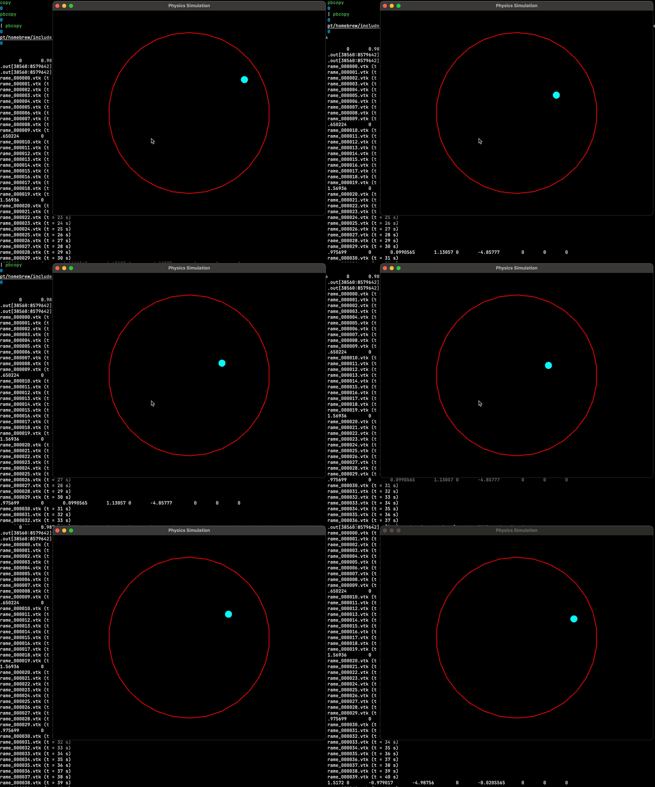
Also, the output directory will have all the egacy vtk files to be visualized in paraview.

Loading the data into paraview#

In both cases, either vtk or csv series of files, we will need to load the files into paraview. The exact paraview command location depends on the machine, but, at the computer room you just run

/mnt/scratch/paraview/bin/paraview &

Then:

Load the data: Browse to the files directory and select the series, which should be shown in a compacted way. Hit apply.
ONLY If you are using the csv files, you need to make them points with attributes. Go to filter and choose the filter Table to Points. Select the right settings and press apply.
Now, add a glyph, of sphere type, and as scale use the field representing the radius.

Now you have your system visualized and if you press play, you can see your system in action!

In paraview you can also perform analysis. For example, you can apply a filter, like only printing particles with some specific speed, or adding some seed histogram in the right, or cut the filter in half and only plot the left part, and so on.

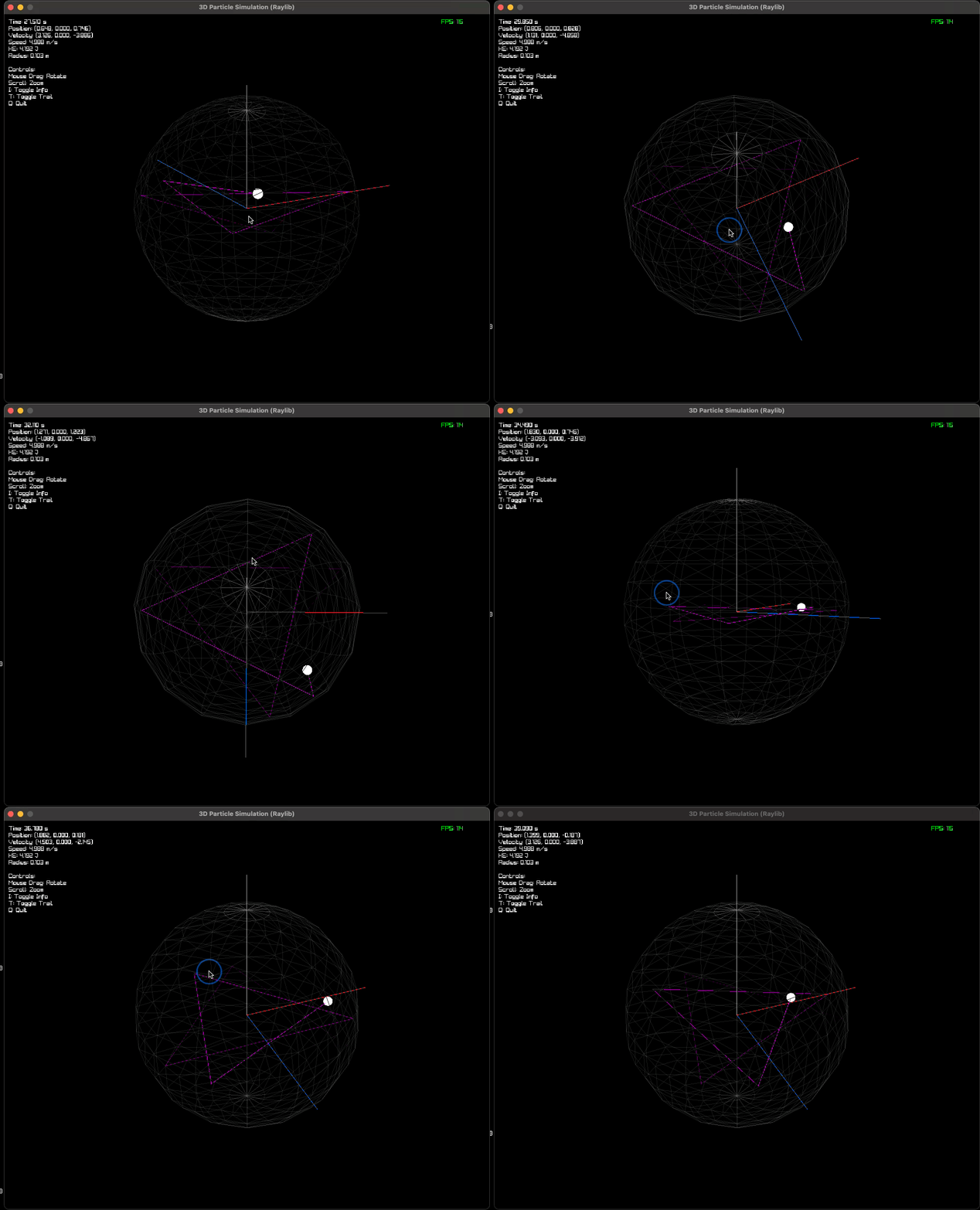
A 3D openGL real time visualization using raylib#

Raylib allows to use opengl without the complexity of manually handling all opengl primitives. Here we implement another class to visualize using raylib, as follows

raylib_visualizer.cpp

#include "raylib_visualizer.h"
#include <raylib.h>
#include <cmath>
#include <sstream>
#include <iomanip>
#include <iostream>

RaylibVisualizer::RaylibVisualizer(unsigned int w, unsigned int h, float scale)
    : width(w), height(h), meters_to_pixels(scale) {
    
    // Initialize raylib window
    InitWindow(static_cast<int>(w), static_cast<int>(h), "3D Particle Simulation (Raylib)");
    SetTargetFPS(120);
    
    // Initialize camera state
    // Camera starts at a distance looking at the origin, slightly elevated
    camera_state.distance = 10.0f;
    camera_state.rotation_x = -0.3f;  // Tilt down slightly
    camera_state.rotation_y = 0.5f;   // Start rotated
    
    // Disable default camera handling (we'll do it manually)
    //DisableCursor();
}

RaylibVisualizer::~RaylibVisualizer() {
    CloseWindow();
}

void RaylibVisualizer::initialize(const std::vector<Particle>& bodies,
                                  float b_radius,
                                  float b_cx,
                                  float b_cy,
                                  float b_cz) {
    boundary_radius = b_radius;
    boundary_cx = b_cx;
    boundary_cy = b_cy;
    boundary_cz = b_cz;
    
    // Clear trajectory
    trajectory.clear();
}

bool RaylibVisualizer::update_and_render(const std::vector<Particle>& bodies,
                                         double time,
                                         double dt) {
    // Handle mouse camera control
    if (IsMouseButtonDown(MOUSE_BUTTON_LEFT)) {
        Vector2 mouse_delta = GetMouseDelta();
        camera_state.rotation_y += mouse_delta.x * 0.01f;
        camera_state.rotation_x -= mouse_delta.y * 0.01f;
        
        // Clamp pitch to avoid gimbal lock
        if (camera_state.rotation_x > 1.4f) camera_state.rotation_x = 1.4f;
        if (camera_state.rotation_x < -1.4f) camera_state.rotation_x = -1.4f;
    }
    
    // Handle mouse wheel for zoom
    float scroll = GetMouseWheelMove();
    camera_state.distance -= scroll * 0.5f;
    if (camera_state.distance < 2.0f) camera_state.distance = 2.0f;
    if (camera_state.distance > 30.0f) camera_state.distance = 30.0f;
    
    // Keyboard shortcuts
    if (IsKeyPressed(KEY_I)) toggle_info();
    if (IsKeyPressed(KEY_T)) toggle_trail();
    if (IsKeyPressed(KEY_Q)) return false;  // Quit
    
    // Update trajectory with current particle position
    if (!bodies.empty()) {
        Vector3 pos = {
            static_cast<float>(bodies[0].R[0]),
            static_cast<float>(bodies[0].R[1]),
            static_cast<float>(bodies[0].R[2])
        };
        trajectory.push_back(pos);
        if (trajectory.size() > MAX_TRAJECTORY_POINTS) {
            trajectory.pop_front();
        }
    }
    
    // Setup camera for 3D rendering
    // Note: Using consistent coordinate order X, Y, Z
    Camera3D camera = {
        .position = {
            boundary_cx + camera_state.distance * std::sin(camera_state.rotation_y) * std::cos(camera_state.rotation_x),
            boundary_cy + camera_state.distance * std::sin(camera_state.rotation_x),
            boundary_cz + camera_state.distance * std::cos(camera_state.rotation_y) * std::cos(camera_state.rotation_x)
        },
        .target = {boundary_cx, boundary_cy, boundary_cz},  // X, Y, Z order (matches particle position)
        .up = {0.0f, 1.0f, 0.0f},
        .fovy = 45.0f,
        .projection = CAMERA_PERSPECTIVE
    };
    
    // Begin 3D rendering
    BeginDrawing();
    ClearBackground(BLACK);
    
    BeginMode3D(camera);
    
    // Draw coordinate axes (for reference)
    DrawLine3D({0.0f, 0.0f, 0.0f}, {3.0f, 0.0f, 0.0f}, RED);    // X axis
    DrawLine3D({0.0f, 0.0f, 0.0f}, {0.0f, 3.0f, 0.0f}, GREEN);  // Y axis
    DrawLine3D({0.0f, 0.0f, 0.0f}, {0.0f, 0.0f, 3.0f}, BLUE);   // Z axis
    
    // Draw boundary sphere (use consistent X, Y, Z coordinate order)
    Vector3 boundary_center = {boundary_cx, boundary_cy, boundary_cz};

    //DrawSphereWires(boundary_center, boundary_radius, 16, 16, GRAY);
    DrawSphereWires(boundary_center, boundary_radius, 16, 16, Fade(GRAY, 0.2f));
    
    // Optional: Draw semi-transparent filled sphere (very faint to not occlude)
    // Commented out to avoid blocking view of particle
    // DrawSphere(boundary_center, boundary_radius, ColorAlpha(DARKBLUE, 0.05f));
    
    // Draw particle trajectory trail
    if (show_trail && trajectory.size() > 1) {
        for (size_t i = 1; i < trajectory.size(); ++i) {
            float alpha = static_cast<float>(i) / trajectory.size();  // Fade out older points
            Color trail_color = ColorAlpha(MAGENTA, alpha * 0.8f);  // Using MAGENTA (raylib pink equivalent)
            DrawLine3D(trajectory[i-1], trajectory[i], trail_color);
        }
    }
    
    // Draw particle and velocity vector
    if (!bodies.empty()) {
        const auto& p = bodies[0];
        Vector3 particle_pos = {
            static_cast<float>(p.R[0]),
            static_cast<float>(p.R[1]),
            static_cast<float>(p.R[2])
        };
        
        float particle_radius = p.rad * 1.0f;  // Scale up for visibility
        
        // Draw solid sphere for particle (bright white for visibility)
        DrawSphere(particle_pos, particle_radius, WHITE);
        
        // // Draw velocity vector as a line (scaled for visibility)
        // float velocity_scale = 0.2f;  // Reduce scale to make it reasonable
        // Vector3 velocity_end = {
        //     particle_pos.x + static_cast<float>(p.V[0]) * velocity_scale,
        //     particle_pos.y + static_cast<float>(p.V[1]) * velocity_scale,
        //     particle_pos.z + static_cast<float>(p.V[2]) * velocity_scale
        // };
        // DrawLine3D(particle_pos, velocity_end, YELLOW);
        
        // // Draw a small sphere at the velocity endpoint
        // DrawSphere(velocity_end, particle_radius * 0.3f, YELLOW);
        
        // Debug: print position occasionally
        if (frame_counter % 60 == 0) {
            double dist = std::sqrt(p.R[0]*p.R[0] + p.R[1]*p.R[1] + p.R[2]*p.R[2]);
            std::cout << "Particle: (" << p.R[0] << ", " << p.R[1] << ", " 
                      << p.R[2] << ") | dist=" << dist << "/" << boundary_radius << "\n";
        }
    }
    
    EndMode3D();
    
    // Draw 2D overlay information
    if (show_info) {
        std::ostringstream oss;
        oss << std::fixed << std::setprecision(3);
        
        if (!bodies.empty()) {
            const auto& p = bodies[0];
            double speed_sq = p.V[0]*p.V[0] + p.V[1]*p.V[1] + p.V[2]*p.V[2];
            double speed = std::sqrt(speed_sq);
            double KE = 0.5 * p.mass * speed_sq;
            
            oss << "Time: " << time << " s\n"
                << "Position: (" << p.R[0] << ", " << p.R[1] << ", " << p.R[2] << ")\n"
                << "Velocity: (" << p.V[0] << ", " << p.V[1] << ", " << p.V[2] << ")\n"
                << "Speed: " << speed << " m/s\n"
                << "KE: " << KE << " J\n"
                << "Radius: " << p.rad << " m\n";
        }
        
        oss << "\nControls:\n"
            << "Mouse Drag: Rotate\n"
            << "Scroll: Zoom\n"
            << "I: Toggle Info\n"
            << "T: Toggle Trail\n"
            << "Q: Quit";
        
        std::string info_text = oss.str();
        DrawText(info_text.c_str(), 10, 10, 12, WHITE);
    }
    
    // Draw FPS counter
    DrawText(TextFormat("FPS: %d", GetFPS()), width - 100, 10, 12, GREEN);
    
    EndDrawing();
    frame_counter++;
    
    return !WindowShouldClose();
}

bool RaylibVisualizer::is_open() const {
    return !WindowShouldClose();
}

main_raylib.cpp

// main_raylib.cpp
// SFML 3 + Raylib with unified visualizer class structure
// g++-15 -std=c++23 -g -I /opt/homebrew/include/ -L /opt/homebrew/lib/ particle.cpp main_raylib.cpp raylib_visualizer.cpp vtk_exporter.cpp -lraylib -lgl
#include "particle.h"
#include "integrator.h"
#include "collider.h"
#include "boundary.h"
#include "raylib_visualizer.h"
#include "vtk_exporter.h"
#include <vector>
#include <map>
#include <string>
#include <iostream>

void initial_conditions(std::vector<Particle>& particles);

int main(int argc, char** argv) {
    std::vector<Particle> bodies;
    bodies.resize(1); // only one particle for now

    // Physics parameters
    std::map<std::string, double> p;
    p["T0"] = 0.0;
    p["TF"] = 100.8767;
    p["DT"] = 0.01;
    p["G"] = 0.0; //-9.81;

    p["RMAX"] = 2.345;

    // Force collider
    Collider collider(p);

    // Time initialization
    TimeIntegrator integrator(p["DT"]);

    // Boundary conditions
    Boundary bc(p["RMAX"], 0.0, 0.0, 0.0, 1.0); // RMAX, CX, CY, CZ, EN

    // Initial conditions and properties
    initial_conditions(bodies);
    collider.computeForces(bodies); // force at t = 0
    integrator.startIntegration(bodies); // start integration algorithm
    
    std::cout << "=== 3D Raylib Simulation Start ===\n";
    std::cout << p["T0"] << "\t";
    bodies[0].print();
    std::cout << "\n";

    // --- VISUALIZATION & I/O SETUP ---
    // Create 3D raylib visualizer
    RaylibVisualizer visualizer(1000, 800, 100.0f);  // width, height, scale
    
    // Initialize visualizer with particles and boundary
    visualizer.initialize(bodies, p["RMAX"], 0.0f, 0.0f, 0.0f);
    
    // Create VTK exporter (same as before)
    VTKExporter vtk_exporter("output");
    vtk_exporter.reset_counter();

    // Time iteration
    const int niter = int((p["TF"] - p["T0"]) / p["DT"]);
    double time = p["T0"];

    std::cout << "Controls:\n"
              << "  Mouse Drag: Rotate camera\n"
              << "  Scroll Wheel: Zoom in/out\n"
              << "  I: Toggle info overlay\n"
              << "  T: Toggle trajectory trail\n"
              << "  Q: Quit\n\n";

    for (int ii = 1; ii < niter; ++ii) {
        // Physics simulation
        collider.computeForces(bodies);
        integrator.timeStep(bodies);
        bc.apply(bodies);
        time += p["DT"];

        // Render (handles window events internally)
        if (!visualizer.update_and_render(bodies, time, p["DT"])) {
            break;  // Window closed
        }

        // Export to VTK every 100 frames
        if (ii % 100 == 0) {
            vtk_exporter.write_frame(bodies, time);
        }

        // Optional: Print to stdout every 1000 frames
        if (ii % 1000 == 0) {
            std::cout << time << "\t";
            bodies[0].print();
            std::cout << "\n";
        }
    }

    std::cout << "=== Simulation Complete ===\n";
    std::cout << "Final time: " << time << " s\n";
    std::cout << "VTK files saved to output/ directory\n";
    
    return 0;
}

void initial_conditions(std::vector<Particle>& particles) {
    particles[0].R[2] = 0.987;    // z is upwards, x to the right
    particles[0].V[0] = 4.9876;   // initial velocity in x
    particles[0].V[2] = 0.0;      // initial velocity in z
    particles[0].rad = 0.103;     // particle radius
    particles[0].mass = 0.337;    // particle mass
}

Output example: