Linear Systems : Matrices, Vectors, eigen systems

In this module we will learn how to solve linear systems which are very common in engineering. Applications are numerous:

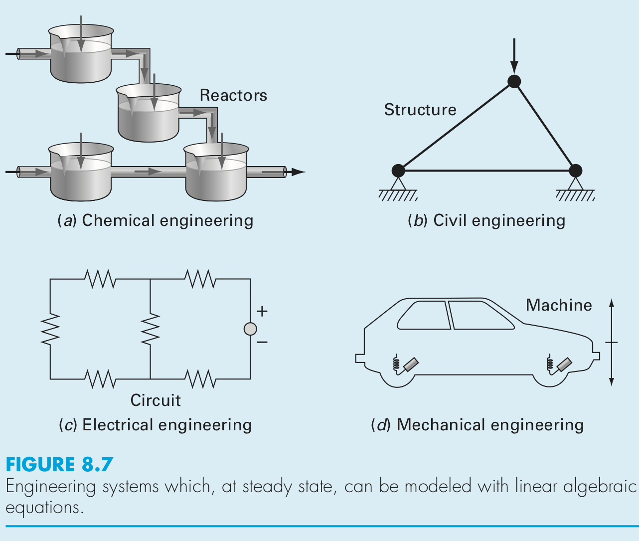
• Civil, chemical, electrical, mechanical, …, engineering

• In biology by using linear algebra to analyze huge data sets regarding protein folding. https://math.stackexchange.com/questions/571109/any-application-of-vector-spaces-in-biology-or-biotechnology

• In genetics to model the evolution of genes.

• Markov chains on industrial processes with applications of matrices and eigen systems.

• Population dynamics.

• Perception of colors.

• Adjacency graphs: https://en.wikipedia.org/wiki/Adjacency_matrix , https://towardsdatascience.com/matrices-are-graphs-c9034f79cfd8

• Other applications: https://www.youtube.com/watch?v=X0HXnHKPXSo

• Matrix operations visualized: https://pytorch.org/blog/inside-the-matrix/ , https://bhosmer.github.io/mm/ref.html

• Matrix and robots: https://www.youtube.com/watch?v=1hG9dx600i8

• Totations http://thenumb.at/Exponential-Rotations/

Tips about matrix computing:

• https://nhigham.com/2022/10/11/seven-sins-of-numerical-linear-algebra/

• http://gregorygundersen.com/blog/2020/12/09/matrix-inversion/

• Quanta magazine: https://www.youtube.com/watch?v=fDAPJ7rvcUw

Ejemplos de rotaciones:

• Particle bouncing

• Plot 3d

# # READ: 
# # https://github.com/vpython/vpython-jupyter?tab=readme-ov-file
# # https://github.com/dragonnomada/vpython-examples?tab=readme-ov-file

import vpython as vp
scene = vp.canvas()
# #vp.sphere()

# axis_x = vp.arrow(pos=vp.vector(0, 0, 0), axis=vp.vector(1, 0, 0), color=vp.color.red)
# axis_y = vp.arrow(pos=vp.vector(0, 0, 0), axis=vp.vector(0, 1, 0), color=vp.color.green)
# axis_z = vp.arrow(pos=vp.vector(0, 0, 0), axis=vp.vector(0, 0, 1), color=vp.color.blue)

# https://www.glowscript.org/docs/VPythonDocs/rotation.html
e = vp.shapes.gear(n=10, radius=0.5)
f = vp.extrusion(path=[vp.vector(0, 0, 0), vp.vector(0, 1, 0)], shape=e)
for ii in range(100):
    f.rotate(angle=vp.radians(10), axis=vp.vector(0, 1, 0))
    vp.sleep(0.05)

---------------------------------------------------------------------------
FileNotFoundError                         Traceback (most recent call last)
Cell In[1], line 15
      7 # #vp.sphere()
      8 
      9 # axis_x = vp.arrow(pos=vp.vector(0, 0, 0), axis=vp.vector(1, 0, 0), color=vp.color.red)
   (...)
     12 
     13 # https://www.glowscript.org/docs/VPythonDocs/rotation.html
     14 e = vp.shapes.gear(n=10, radius=0.5)
---> 15 f = vp.extrusion(path=[vp.vector(0, 0, 0), vp.vector(0, 1, 0)], shape=e)
     16 for ii in range(100):
     17     f.rotate(angle=vp.radians(10), axis=vp.vector(0, 1, 0))

File /opt/hostedtoolcache/Python/3.11.11/x64/lib/python3.11/site-packages/vpython/vpython.py:3946, in extrusion.__init__(self, **args)
   3943     if attr in args and isinstance(args[attr],list) and len(args[attr]) != self._pathlength:
   3944         raise AttributeError("The "+attr+" list must be the same length as the list of points on the path ("+str(self._pathlength)+").")
-> 3946 super(extrusion, self).setup(args)
   3948 self.canvas._compound = self # used by event handler to update pos and size
   3949 _wait(self.canvas)

File /opt/hostedtoolcache/Python/3.11.11/x64/lib/python3.11/site-packages/vpython/vpython.py:612, in standardAttributes.setup(self, args)
    611 def setup(self, args):
--> 612     super(standardAttributes, self).__init__()
    613     self._constructing = True  ## calls to setters are from constructor
    615     objName = self._objName = args['_objName']  ## identifies object type

File /opt/hostedtoolcache/Python/3.11.11/x64/lib/python3.11/site-packages/vpython/vpython.py:265, in baseObj.__init__(self, **kwargs)
    262 if not (baseObj._view_constructed or
    263         baseObj._canvas_constructing):
    264     if _isnotebook:
--> 265         from .with_notebook import _
    266     else:
    267         from .no_notebook import _

File /opt/hostedtoolcache/Python/3.11.11/x64/lib/python3.11/site-packages/vpython/with_notebook.py:71
     66         except PermissionError:
     67             #logging.info("PermissionError: Unable to install /vpython_data directory and files for VPython on JupyterLab")
     68             pass
---> 71 if ('nbextensions' in os.listdir(jd)) and (notebook.__version__ <= '6.5.5'):
     72     ldir = os.listdir(nbdir)
     73     if ('vpython_data' in ldir and len(os.listdir(nbdata)) == datacnt and
     74        'vpython_libraries' in ldir and len(os.listdir(nblib)) == libcnt and
     75         'vpython_version.txt' in ldir):

FileNotFoundError: [Errno 2] No such file or directory: '/home/runner/.local/share/jupyter'

Linear systems

How to adapt to python the following matrix system?

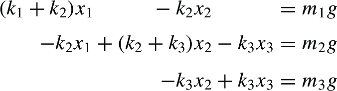
Write this as a linear system \(A\vec x = \vec b\), with unknows \(x_1, x_2, x_3\)

A = (k1+k2 -k2 0 -k2 k2+k3 -k3 0 -k3 k3)

[[k1 + k2, -k2  , 0  ],
 [-k2    , k2+k3, -k3],
 [0      , -k3  , k3]]

x = (x1 x2 x3)

b = (m1g m2g m3g)

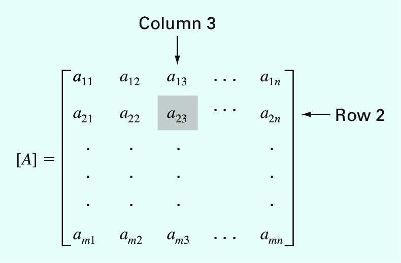
How to index a Matrix? NOTE: Python indexes start at 0

For a discussion about starting at zero see: https://news.ycombinator.com/item?id=32581721

Defining matrices in python

DO NOT USE PYTHON LISTS!

Scipy

See https://docs.scipy.org/doc/numpy-1.17.0/reference/generated/numpy.array.html#numpy.array

import numpy as np
A = np.array([[1, 2],  # primera fila, indice es 0
              [3, 4]]) # Segunda fila, indice es 1
print(A[0][1])
print(f"Matrix : \n", A)
#
A = np.array([1, 2, 3, 4]).reshape(2,2)
print("Matrix : \n", A)
print("A[1,0] : \n", A[1,0])
print("A[1][0] : \n", A[1][0])

print("A[:,-1] : \n", A[:,-1])

Matrix operations

Add, substract, multiply, etc

import numpy as np
a = np.array([[1, 2],[3, 4]])
b = np.array([[5, -1], [-3, 24]])
c = a+b # sum
print(c)
c = a*b # Multiplication
print(c)
c = a/b # divide element by element
print(c)
print(c.max())
print(c.min())
print(b/b)

Solving linear systems \(A\vec x= \vec b\)

Solve the following system:

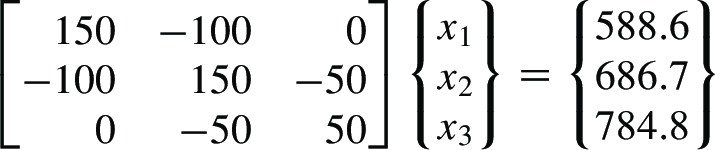
import numpy as np

A = np.array([[150, -100, 0], 
              [-100, 150, -50], 
              [0, -50, 50]])
b = np.array([588.6, 686.7, 784.8])
x = np.linalg.solve(A, b) # magic
print("Solution: \n", x)
# confirm
print("Delta:\n", A.dot(x) - b)

import numpy as np

#np.random.seed(10) # Play with this value

N = 1000

A = np.random.rand(N,N)
b = np.random.rand(N)
x = np.linalg.solve(A, b) # magic
print("Solution: \n", x[:10])
# confirm
#print("Delta:\n", A.dot(x) - b)

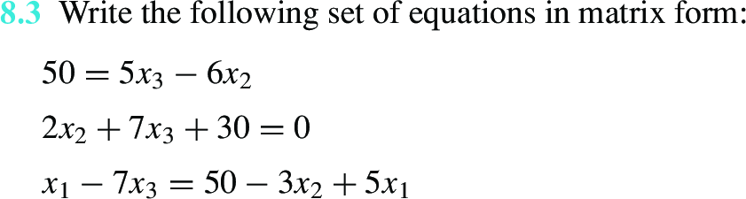
Exercise: Rewrite and solve the following system

# YOUR CODE HERE
raise NotImplementedError()

assert np.all(np.isclose(x, np.array([-17.01923077,  -9.61538462,  -1.53846154])))

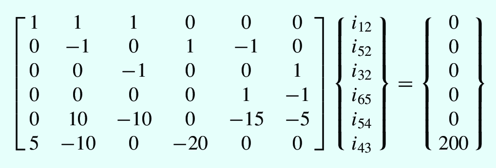
Exercise: Rewrite and solve the following system

Extra: Can you measure the time spent in the computation? (google for timer or timeit in python)

# YOUR CODE HERE
raise NotImplementedError()

assert np.all(np.isclose(x, np.array([ 6.15384615, -4.61538462, -1.53846154, -6.15384615, -1.53846154, -1.53846154])))

Exercise: Solve and plot the following system

\[ \frac{-2.3x_1}{5} + x_2 = 1.1 \]

\[-0.5x_1 + x_2 = 1 \]

Plot the system of equations and check whether this solution is or not special. Compute the quantity np.linalg.cond

# YOUR CODE HERE
raise NotImplementedError()

Exercise: Simulating temperature

• Temperature discretized

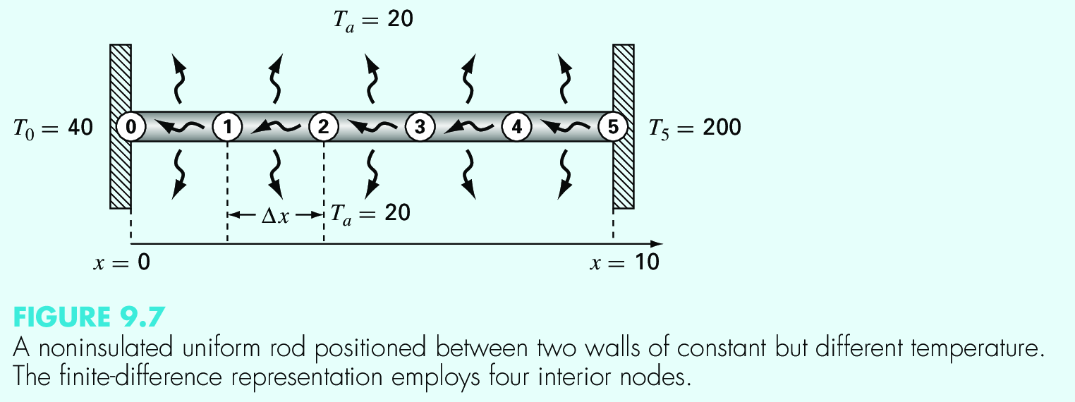
• System of equations

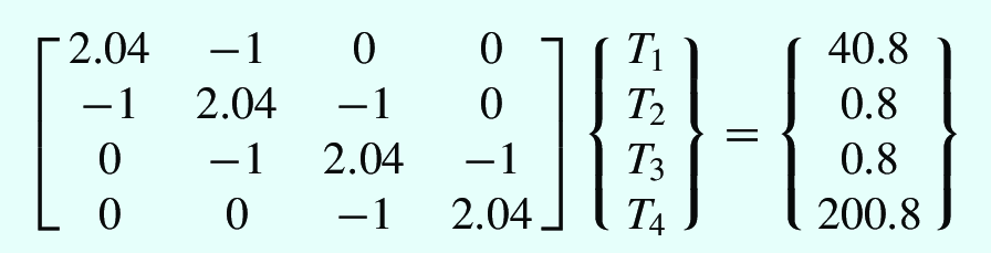
# YOUR CODE HERE
raise NotImplementedError()

Exercise

How does the computing time grows with the matrix size?

# YOUR CODE HERE
raise NotImplementedError()

Computing inverse matrices

See : https://docs.scipy.org/doc/scipy/reference/generated/scipy.linalg.inv.html#scipy.linalg.inv

You can watch: https://www.youtube.com/watch?v=uQhTuRlWMxw

%time
from scipy import linalg
import numpy as np
A = np.array([[1., 2.], 
              [3., 4.]])
B = linalg.inv(A) # magic
#print("B : \n", B)
# verify
#print("A A^-1 : \n", A.dot(B))

%%time
from scipy import linalg
import numpy as np
N = 1000
A = np.random.rand(N, N)
B = linalg.inv(A) # magic
#print("B : \n", B)
# verify
#print("A A^-1 : \n", A.dot(B))

The condition number

The number

\[\kappa = ||A|| ||A^{-1}||\]

is called the condition number of a matrix. Ideally it is \(1\). If \(\kappa\) is much larger than one, the matrix is ill-conditioned and the solution might have a lot of error.

Compute the condition number of the following matrix:

(10)\[\begin{equation} A = \begin{bmatrix} 1.001 & 0.001\\ 0.000 & 0.999 \end{bmatrix} \end{equation}\]

Plot the associate system to check for the result

from scipy import linalg
import numpy as np
A = np.array([[1.001, 0.001],
                [0.000, 0.999]])
kappa = linalg.norm(A)*linalg.norm(linalg.inv(A))
print(f"{kappa = }")

Exercise

How does the computing time grows with the matrix size?

from scipy import linalg
import numpy as np
import time # use time.process_time_ns() , compare with monotonic_ns()

MINSIZE=1
MAXSIZE=5000
NSAMPLES=10
data = np.zeros((NSAMPLES, 3))
# YOUR CODE HERE
raise NotImplementedError()

# YOUR CODE HERE
raise NotImplementedError()

# pip install heat
%load_ext heat

%%heat
# YOUR CODE HERE
raise NotImplementedError()

Improve this by taking at least 10 time samples per matrix size and computing the statistics

Eigen values and eigen vectors

The eigen-values \({\lambda_i}\) and eigen-vectors \({x}\) of a matrix satisfy the equation

\[ A\vec x = \lambda \vec x \]

The eigen-vectors form a basis where the matrix can be diagonalized. In general, computing the eigen vectors and aeigenvalues is hard, and they can also be complex.

For a more visual introduction watch: https://www.youtube.com/watch?v=PFDu9oVAE-g

REF: https://www.reddit.com/r/math/comments/b7ou6t/3blue1brown_overview_of_differential_equations/

# See : https://docs.scipy.org/doc/scipy/reference/generated/scipy.linalg.eig.html#scipy.linalg.eig
import numpy as np
from scipy import linalg
#A = np.array([[0., -1.], [1., 0.]])
#A = np.array([[1, 0.], [0., 2.]])
A = np.array([[2, 5, 8, 7], [5, 2, 2, 8], [7, 5, 6, 6], [5, 4, 4, 8]])
sol = linalg.eig(A) # magic
print("Eigen-values: ", sol[0])
print("Eigen-vectors:\n", sol[1])
# verify
print("Verification: ", A.dot(sol[1][:, 0]) - sol[0][0]*sol[1][:, 0])

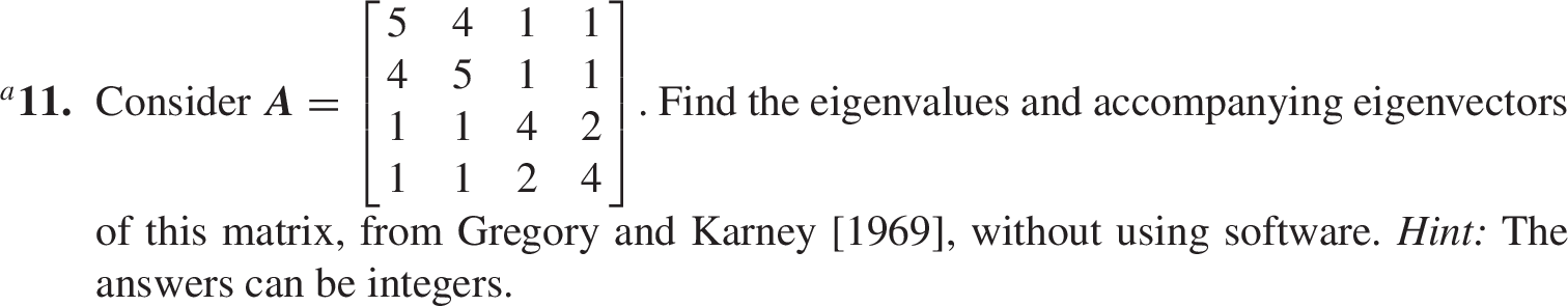
Exercise

Find the eigen-values and eigen-vectors for the following system

# YOUR CODE HERE
raise NotImplementedError()

Exercise

How does the computing time grows with the matrix size?

# YOUR CODE HERE
raise NotImplementedError()

# YOUR CODE HERE
raise NotImplementedError()

Problems

Linear System

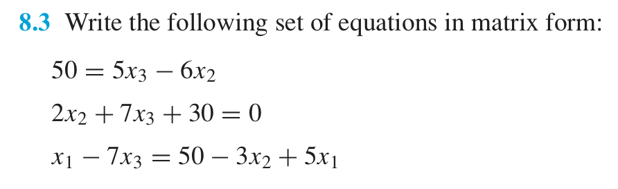
# YOUR CODE HERE
raise NotImplementedError()

Rotation matrix

Let \(\vec x = (a, b)\) be a two-dimensional vector. Write a matrix that rotates the vector by 90 degrees. Use matrix multiplication to check your results.

# YOUR CODE HERE
raise NotImplementedError()

Thick lens (Boas, 3.15.9)

The next matrix is used when discussing a thick lens in air

(11)\[\begin{equation} A = \begin{pmatrix} 1 & (n-1)/R_2\\ 0 & 1 \end{pmatrix} \begin{pmatrix} 1 & 0\\ d/n & 1 \end{pmatrix} \begin{pmatrix} 1 & -(n-1)/R_1\\ 0 & 1 \end{pmatrix}, \end{equation}\]

where \(d\) is the thickness of the lens, \(n\) is the refraction index, and \(R_1\) and \(R_2\) are the curvature radius. Element \(A_{12}\) is equal to \(-1/f\), where \(f\) is the focal distance. Evaluate \(\det A\) and \(1/f\) as functions of \(n \in [1, 3]\).

# YOUR CODE HERE
raise NotImplementedError()

System of reactors

System	Model

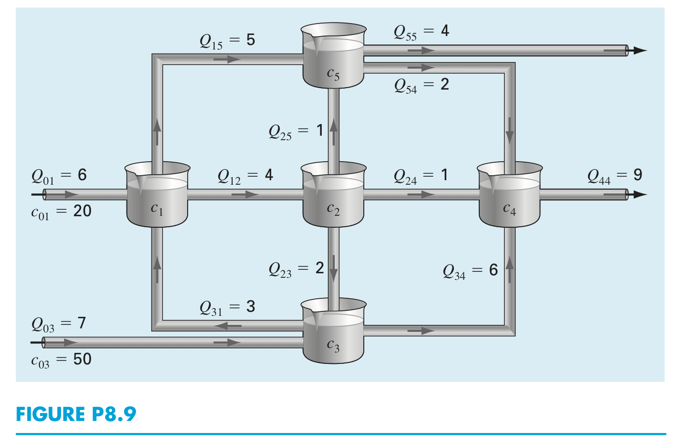
# YOUR CODE HERE
raise NotImplementedError()

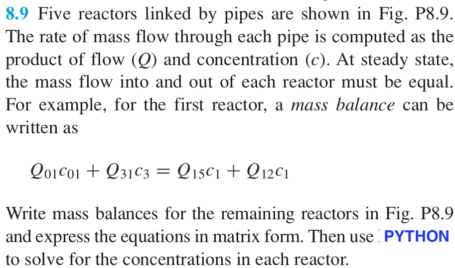
Products production

# YOUR CODE HERE
raise NotImplementedError()

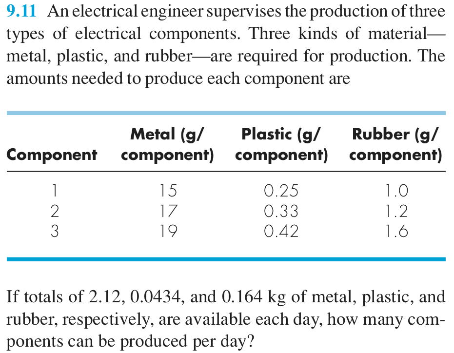
Teaching distribution

# YOUR CODE HERE
raise NotImplementedError()

GPA

Statement	Table

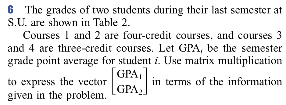
# YOUR CODE HERE
raise NotImplementedError()

Payments

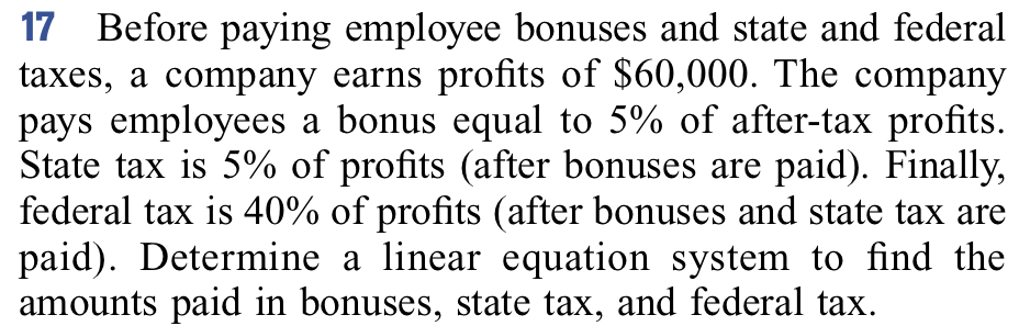
# YOUR CODE HERE
raise NotImplementedError()