
Partial Differential equations: Finite differences#
REFS:
Franklin, Computational methods for Physics
Landau y Paez, Computational physics
Boudreau et al, Applied Computational Physics
The following is an example of an elliptical differential equation, determined by the boundary conditions :
In 2D, there are several solutions and the actual one depends on the boundary conditions. For example, for the Laplace equation you have
as solutions.
A finite difference method discretizes the derivatives on a grid. For instance, using the central difference it is possible to rewrite the 2D Poisson equation as (Laplace equation corresponds to \(\rho = 0\) )
which can be rewritten as (let’s assume \(\Delta x = \Delta y = \Delta\))
and, therefore
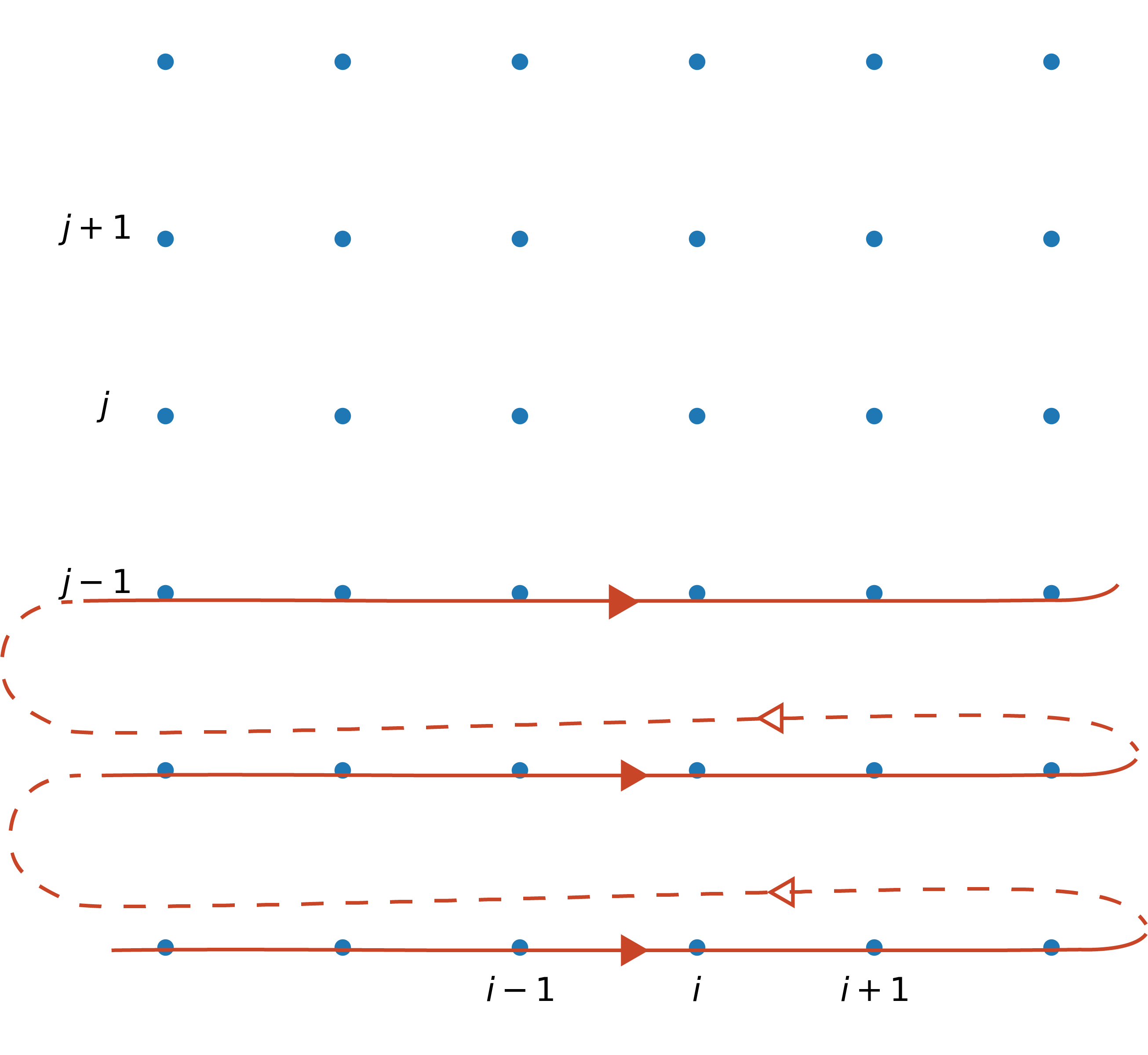
This can be seen in two ways: as a matrix equation or as an equation showing that the value at a given position, \(V_{i, j}\), is kind of an average of the surrounding neighbors and the source term (Jacobi method), as seen (ref: https://barbagroup.github.io/essential_skills_RRC/laplace/1/#laplaces-equation)

The first approach can be solved by using the typical matrix methods (on the banded matrix obtained), while the second one gives raise to the relaxation method, where you sweep the matrix several times until stabilization is achieved.
Relaxation solution#
Let’s solve the Laplace problem (\(\rho = 0\)) using both methods with a simple example. Fix the boundaries as
with \(x, y \in [0, 1]\), and \(a \) any value on the border. These are called Dirichlet boundary conditions (where you specify the function values at the boundary). Finally, use at least \(N_x = N_y = 25\), so \(\Delta = 1/25\), \(x_i = x_0 + i\Delta, y_j = y_0 + j\Delta\). We need to solve the equation
To do so, we apply this relationship to each point in the grid, without overwriting the boundary conditions, and we do that until the values are not changing much. Firs, let’s define the problem conditions (to be changed later)
# Global problem definition
import numpy as np
def setup_problem(N):
    XMIN = 0.0
    YMIN = 0.0
    DELTA = 1.0/N
    X = XMIN + DELTA*np.arange(0, N)
    Y = XMIN + DELTA*np.arange(0, N)
    return X, Y
Now create a function for the boundary conditions
# Boundary conditions
def bc(matrix, x, y):
    # YOUR CODE HERE
    raise NotImplementedError()
And this will be a simple example for single iteration step. In this case, we are avoiding the external walls since they are boundary conditions. We are using the fast numpy notation (see also https://becksteinlab.physics.asu.edu/learning/76/phy494-computational-physics?wchannelid=bp7lsp6dmx&wmediaid=284owsl3dp), but of course you can use loops (specially for more complex boundary problems)
# Full iteration using for loops
def jacobiITER(matrix):
    # YOUR CODE HERE
    raise NotImplementedError()
# Full iteration using only numpy indexing
def jacobi(matrix):
    # YOUR CODE HERE
    raise NotImplementedError()
Finally, let’s perform some iterations to check if the system is converging somewhere
import time
def solve_system(N, niter, iter_method):
    X, Y = setup_problem(N)
    V = np.zeros((N, N))
    bc(V, X, Y)
    # Example iteration
    for step in range(niter):
        #print(V)
        t0 = time.time()
        iter_method(V)
        t1 = time.time()
        print(f"Total time iterating: {t1-t0}")
        #print(V)
        #print()
solve_system(N=500, niter=10, iter_method=jacobiITER)
#solve_system(N=500, niter=10, iter_method=jacobi)
---------------------------------------------------------------------------
NotImplementedError                       Traceback (most recent call last)
Cell In[6], line 1
----> 1 solve_system(N=500, niter=10, iter_method=jacobiITER)
      2 #solve_system(N=500, niter=10, iter_method=jacobi)

Cell In[5], line 5, in solve_system(N, niter, iter_method)
      3 X, Y = setup_problem(N)
      4 V = np.zeros((N, N))
----> 5 bc(V, X, Y)
      6 # Example iteration
      7 for step in range(niter):
      8     #print(V)

Cell In[2], line 4, in bc(matrix, x, y)
      2 def bc(matrix, x, y):
      3     # YOUR CODE HERE
----> 4     raise NotImplementedError()

NotImplementedError:
Or let’s check it graphically
import matplotlib.pyplot as plt
import numpy as np
def solve_system(N, niter, iter_method, NDISPLAY=2):
    # figs setup
    NCOLS = 4
    NROWS = int(((niter/NDISPLAY)/NCOLS))
    if ((niter/NDISPLAY)%NCOLS) != 0:
        NROWS += 1
    fig, ax = plt.subplots(NROWS, NCOLS, sharex=True, sharey=True, figsize=(15, 15))
    ax = ax.flatten()
    # Problem setup
    X, Y = setup_problem(N)
    V = np.zeros((N, N))
    bc(V, X, Y)
    # Example iteration
    idisplay= 0
    for step in range(niter):
        if step%NDISPLAY == 0:
            # ax[idisplay].set_title(step)
            # ax[idisplay].imshow(V)
            ax[idisplay].set_aspect('equal', 'box')
            ax[idisplay].pcolormesh(V)
            ax[idisplay].set_title(f"niter={niter}")
            CS = ax[idisplay].contour(V, cmap='Blues')
            ax[idisplay].clabel(CS, CS.levels, inline=True)
            idisplay += 1
        iter_method(V)
solve_system(N=20, niter=200, iter_method=jacobi, NDISPLAY=20)
To have a quantitative relaxation index, we could compare the new values with the old ones, so let’s redefine the iteration step method to return the estimator
def jacobi2(matrix):
    matrix_old = matrix.copy() # Might be slow, creates copies all the time
    # YOUR CODE HERE
    raise NotImplementedError()
def solve_system(N, niter, iter_method):
    X, Y = setup_problem(N)
    V = np.zeros((N, N))
    bc(V, X, Y)
    diff = np.zeros(niter)
    # Example iteration
    for step in range(niter):
        diff[step] = iter_method(V)
    return diff
diff = solve_system(N=5, niter=200, iter_method=jacobi2)
plt.plot(diff)
plt.xscale("log")
plt.yscale("log")
Notice that the convergence depends strongly on the space resolution:
for N in [5, 7, 10, 20, 50 , 100, 200, 500]:
    print(N)
    diff = solve_system(N=N, niter=1000, iter_method=jacobi2)
    plt.plot(diff, label=f"{N=}")
plt.xscale("log")
plt.yscale("log")
plt.legend()
We can also use the Gauss-Seidel approach by overwriting the original matrix (and even SOR) to speed up convergence
You might need to use a for loop
def gs(matrix):
    matrix_old = matrix.copy() # Might be slow, creates copies all the time
    N = matrix.shape[0]
    # YOUR CODE HERE
    raise NotImplementedError()
for N in [5, 7, 10, 20, 50 , 100, 200, 500]:
    print(N)
    diff = solve_system(N=N, niter=1000, iter_method=gs)
    plt.plot(diff, label=f"{N=}")
plt.xscale("log")
plt.yscale("log")
plt.legend()
A performance discussion#
But this loop version is very slow. When you need to optimize something, you need to measure it (using profilers). Here we will use https://jakevdp.github.io/PythonDataScienceHandbook/01.07-timing-and-profiling.html and https://mortada.net/easily-profile-python-code-in-jupyter.html .
%%timeit
tmp = solve_system(N=50, niter=100, iter_method=gs)
We can optimize with numba (see https://stackoverflow.com/questions/61161072/optimizing-vectorized-operations-made-by-sections-in-numpy):
#!conda install -y numba
#!pip install -y numba
!uv pip install numba numpy==2.0
# YOUR CODE HERE
raise NotImplementedError()
%%timeit
tmp = solve_system(N=50, niter=100, iter_method=gs_opt)
for N in [5, 7, 10, 20, 50 , 100, 200, 500]:
    print(N)
    diff = solve_system(N=N, niter=1000, iter_method=gs_opt)
    plt.plot(diff, label=f"{N=}")
plt.xscale("log")
plt.yscale("log")
plt.legend()
Plotting the solution#
Now let’s plot the actual solution
def solve_system(N, niter, iter_method):
    X, Y = setup_problem(N)
    V = np.zeros((N, N))
    bc(V, X, Y)
    diff = np.zeros(niter)
    # Example iteration
    for step in range(niter):
        diff[step] = iter_method(V)
    return V
fig, ax = plt.subplots(2, 3, figsize=(8,6))
ax = ax.flatten()
for ii, niter in enumerate([5, 10, 100, 1000, 5000, 10000]):
    V = solve_system(N=50, niter=niter, iter_method=gs_opt)
    ax[ii].set_aspect('equal', 'box')
    ax[ii].pcolormesh(V)
    ax[ii].set_title(f"niter={niter}")
    CS = ax[ii].contour(V, cmap='Blues')
    ax[ii].clabel(CS, CS.levels, inline=True)
fig.tight_layout()
fig.savefig("potential.pdf")
Exercise: Plane capacitor#
Now , besides the given boundary conditions, add two lines representing a plane capacitor, with opposite voltages of \(\pm 3\) volts, with length \(2L_y/3\), at \(L_x/3\) and \(2L_x/3\). Plot the final solution as a 2D map and as a 3D map.
# YOUR CODE HERE
raise NotImplementedError()
Exercise: circular ring#
Now , besides the given boundary conditions, add a circular ring with constant voltage of 3 volts and radius \(L_x/4\). Plot the final solution as a 2D map and as a 3D map.
# YOUR CODE HERE
raise NotImplementedError()
Exercise: Plot the electrical field#
For any of the previous examples, use (for example) a quiver plot to plot the electric field, defined as
See https://nbviewer.org/urls/www.numfys.net/media/notebooks/relaxation_methods.ipynb
# YOUR CODE HERE
raise NotImplementedError()
Exercise: Add two square charges#
Solve the Poisson equation with two square charges of size \(L_x/10\) on the diagonal. Use \(\epsilon_0 = 1\)
Exercise: Implement over-relaxation#
Calibrate \(\omega\) (see https://en.wikipedia.org/wiki/Successive_over-relaxation)
from numba import jit
@jit
def gs_sor_opt(matrix, omega):
    matrix_old = matrix.copy() # Might be slow, creates copies all the time
    gs_opt(matrix)
    rij = matrix - matrix_old
    matrix = matrix_old + omega*rij
    rij = matrix - matrix_old
    diff = np.linalg.norm(rij)
    return diff
    #return gs_opt(matrix)
#for N in [5, 7, 10, 20, 50 , 100, 200, 500]:
for N in [5]:
    print(N)
    OMEGA=1.9
    diff = solve_system(N=N, niter=1000, iter_method=lambda m: gs_sor_opt(m, OMEGA))
    plt.plot(diff, label=f"{N=}")
plt.xscale("log")
plt.yscale("log")
plt.legend()
Exercise: Stop after tolerance is achieved#
Modify the iteration procedure to stop after some given precision has been achieved
# YOUR CODE HERE
raise NotImplementedError()