
Numerical libraries for PDEs#
Give n the enormous complexity that PDE can present, there are scientific libraries targeted to their solutions. Here we will show just a few to highlight their use. In particular, two libraries that use the powerful finite element method to solve PDE in complex geometries, will be shown at the end.
findiff#
https://github.com/maroba/findiff
uv pip install findiff
%matplotlib inline
#!/usr/bin/env python3

from findiff import Diff, Id, PDE, FinDiff, BoundaryConditions
import numpy as np


shape = (100, 100)
x, y = np.linspace(0, 1, shape[0]), np.linspace(0, 1, shape[1])
dx, dy = x[1]-x[0], y[1]-y[0]
X, Y = np.meshgrid(x, y, indexing='ij')

L = FinDiff(0, dx, 2) + FinDiff(1, dy, 2)
f = np.zeros(shape)

bc = BoundaryConditions(shape)
bc[1,:] = FinDiff(0, dx, 1), 0  # Neumann BC
bc[-1,:] = 300. - 200*Y   # Dirichlet BC
bc[:, 0] = 300.   # Dirichlet BC
bc[1:-1, -1] = FinDiff(1, dy, 1), 0  # Neumann BC

pde = PDE(L, f, bc)
u = pde.solve()
---------------------------------------------------------------------------
ModuleNotFoundError                       Traceback (most recent call last)
Cell In[1], line 4
      1 get_ipython().run_line_magic('matplotlib', 'inline')
      2 #!/usr/bin/env python3
----> 4 from findiff import Diff, Id, PDE, FinDiff, BoundaryConditions
      5 import numpy as np
      8 shape = (100, 100)

ModuleNotFoundError: No module named 'findiff'
import matplotlib.pyplot as plt
plt.imshow(u)
Py-pde#
uv pip install py-pde
import pde

grid = pde.UnitGrid([64, 64])                 # generate grid
state = pde.ScalarField.random_uniform(grid)  # generate initial condition

eq = pde.DiffusionPDE(diffusivity=0.1)        # define the pde
result = eq.solve(state, t_range=10)          # solve the pde
result.plot()                                 # plot the resulting field
import numpy as np

from pde import CartesianGrid, solve_laplace_equation

grid = CartesianGrid([[0, 2 * np.pi], [0, 2 * np.pi]], 64)
bcs = {"x": {"value": "sin(y)"}, "y": {"value": "sin(x)"}}

res = solve_laplace_equation(grid, bcs)
res.plot()
import pde

grid = pde.UnitGrid([32, 32])  # generate grid
state = pde.ScalarField.random_uniform(grid)  # generate initial condition

storage = pde.MemoryStorage()

trackers = [
    "progress",  # show progress bar during simulation
    "steady_state",  # abort when steady state is reached
    storage.tracker(interrupts=1),  # store data every simulation time unit
    pde.PlotTracker(show=True),  # show images during simulation
    # print some output every 5 real seconds:
    pde.PrintTracker(interrupts=pde.RealtimeInterrupts(duration=5)),
]

eq = pde.DiffusionPDE(0.1)  # define the PDE
eq.solve(state, 3, dt=0.1, tracker=trackers)

for field in storage:
    print(field.integral)
MFEM#
Although it is c++, it has a python wrapper
https://mfem.org/
https://github.com/mfem/PyMFEM
https://mfem.org/examples/
https://colab.research.google.com/github/mfem/pymfem/blob/master/examples/jupyter/ex1.ipynb
https://colab.research.google.com/github/mfem/pymfem/blob/master/examples/jupyter/ex9.ipynb
https://github.com/mfem/PyMFEM/tree/master/examples
Only works on linux
uv pip install pip
pip install mfem # be sure to be used the uv installed pip
(for advanced options, like parallelization, you should download the sources and compile with the right options)
import mfem.ser as mfem

# Create a square mesh
mesh = mfem.Mesh(10, 10, "TRIANGLE")

# Define the finite element function space
fec = mfem.H1_FECollection(1, mesh.Dimension())   # H1 order=1
fespace = mfem.FiniteElementSpace(mesh, fec)

# Define the essential dofs
ess_tdof_list = mfem.intArray()
ess_bdr = mfem.intArray([1]*mesh.bdr_attributes.Size())
fespace.GetEssentialTrueDofs(ess_bdr, ess_tdof_list)

# Define constants for alpha (diffusion coefficient) and f (RHS)
alpha = mfem.ConstantCoefficient(1.0)
rhs = mfem.ConstantCoefficient(1.0)

"""
Note
-----
In order to represent a variable diffusion coefficient, you
must use a numba-JIT compiled function. For example:

>>> @mfem.jit.scalar
>>> def alpha(x):
>>>     return x+1.0
"""

# Define the bilinear and linear operators
a = mfem.BilinearForm(fespace)
a.AddDomainIntegrator(mfem.DiffusionIntegrator(alpha))
a.Assemble()
b = mfem.LinearForm(fespace)
b.AddDomainIntegrator(mfem.DomainLFIntegrator(rhs))
b.Assemble()

# Initialize a gridfunction to store the solution vector
x = mfem.GridFunction(fespace)
x.Assign(0.0)

# Form the linear system of equations (AX=B)
A = mfem.OperatorPtr()
B = mfem.Vector()
X = mfem.Vector()
a.FormLinearSystem(ess_tdof_list, x, b, A, X, B)
print("Size of linear system: " + str(A.Height()))

# Solve the linear system using PCG and store the solution in x
AA = mfem.OperatorHandle2SparseMatrix(A)
M = mfem.GSSmoother(AA)
mfem.PCG(AA, M, B, X, 1, 200, 1e-12, 0.0)
a.RecoverFEMSolution(X, b, x)

# Extract vertices and solution as numpy arrays
verts = mesh.GetVertexArray()
sol = x.GetDataArray()

# Plot the solution using matplotlib
import matplotlib.pyplot as plt
import matplotlib.tri as tri

triang = tri.Triangulation(verts[:,0], verts[:,1])

fig, ax = plt.subplots()
ax.set_aspect('equal')
tpc = ax.tripcolor(triang, sol, shading='gouraud')
fig.colorbar(tpc)
plt.show()
Fenics#
https://fenicsproject.org/
https://fenicsproject.org/documentation/
https://docs.fenicsproject.org/dolfinx/v0.9.0/python/demos.html
https://jsdokken.com/dolfinx-tutorial/chapter1/fundamentals.html
https://docs.pyvista.org/
Installation is much more complicated than
uv pip install fenics dolphin mpi4py
It is better to use a docker container or use the binder setups
Example: 2D poisson equation
Notation and method intro: https://jsdokken.com/dolfinx-tutorial/chapter1/fundamentals.html
Implementation (use binder) : https://jsdokken.com/dolfinx-tutorial/chapter1/fundamentals_code.html
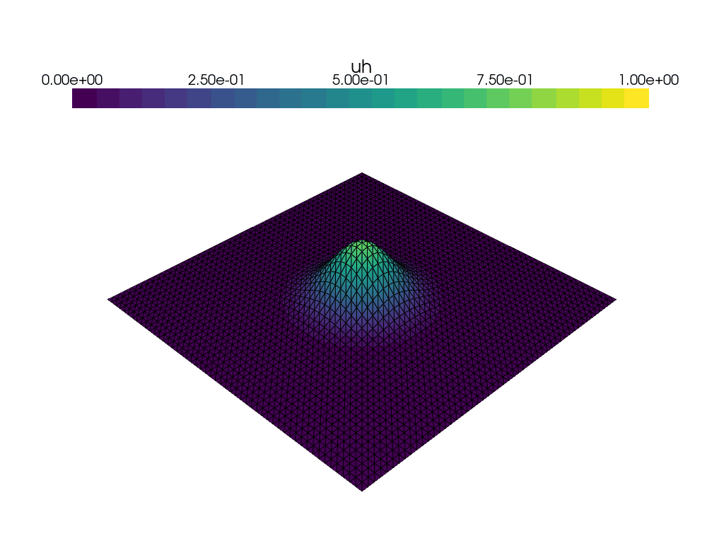
From : https://jsdokken.com/dolfinx-tutorial/chapter2/diffusion_code.html
To Check#
https://getfem-examples.readthedocs.io/en/latest/demo_unit_disk.html
https://www.pygimli.org/_tutorials_auto/2_modelling/plot_2-mod-fem.html
https://flocode.substack.com/p/049-pynite-01-introduction-to-finite
https://bleyerj.github.io/comet-fenicsx/
https://gmshmodel.readthedocs.io/en/latest/