
Molecular Dynamics#
https://github.com/hannorein/rebound
Molecular dynamics (MD)is a simulation technique that is applied from actual molecules to systems as large as planetary rings (for granular systems and beyond it is known as Discrete Element Method). The key is to have discrete bodies that interact under some given potential fields or forces and from that to integrate the equations of motion. To apply a MD simulation you will need to
define a body: Usually done using a class/struct. Examples are atoms, molecules, grains of sand, rocks, blocks of ice, etc.
define forces among bodies: Those can be only external (gravity, potential fields), or by contact (repulsion, friction, damping), etc. Usually modeled using a Collider class/struct or similar.
define an integration technique: this will allow to solve the dynamic equations. Examples are Verlet, Velocity Verlet, Leap-Frog, Symplectic algorithms, RESPA, etc. Can be modeled as simple functions or as class/struct for more complex situations.
Of course many details are left out in this short introduction (pre-processing or sample preparation, optimization with Verlet lists and/or cell lists, rotations, compund bodies, post-processing and analysis, etc).
Some examples of HPC systems for Molecular Dynamics at the level of molecules are lammps, grommacs, and many more. For the Discrete Element Method, we have lammps (with the granular package), liggghts, mechsys, mercury dpm, Yade, Altair, Rocky, etc
In the following we will focus MD applied to macroscopic bodies (in the final projects you will be able to use some of the previously mentioned packages and to apply it to different systems).
Defining the body#
We will start by simulating a particle under the gravity force. The basic attributes to for a particle of this kind would be
mass (scalar)
Position, velocity and force (vectors) Other possible like the radius are not as relevant now since we are focusing only on Center of Mass dynamics. Let’s define the body class
%%writefile body.py
import numpy as np
class Body:
    """
    Class to model a simple point body
    """
    def __init__(self, R0, V0, m0, r0 = 0.0): # constructor
        self.mass = m0
        self.rad = r0
        self.R = np.array(R0)
        self.V = np.array(V0)
        self.F = np.zeros(3)


if __name__ == "__main__":
    R0 = np.array([0, 0.9, 0.0])
    V0 = np.array([0.98, 1.23, 0.0])
    mass = 0.4343
    body = Body(R0, V0, mass)
    print(body.mass)
    print(body.V[1])
Overwriting body.py
To use it, let’s just instantiate the class
R0 = np.array([0, 0.9, 0.0])
V0 = np.array([0.98, 1.23, 0.0])
mass = 0.4343
body = Body(R0, V0, mass)
---------------------------------------------------------------------------
NameError                                 Traceback (most recent call last)
Cell In[2], line 1
----> 1 R0 = np.array([0, 0.9, 0.0])
      2 V0 = np.array([0.98, 1.23, 0.0])
      3 mass = 0.4343

NameError: name 'np' is not defined
Forces#
For now, we will just add gravity, so our Collider class will be very simple, with only some parameters
%%writefile collider.py
import numpy as np
class Collider:
    """
    Class to compute forces on each body
    """
    # Parameters
    G = np.array([0.0, -9.81, 0.0])
    B = 3.9
    K = 1000.345

    # Functions
    def computeForce(self, body): # For now operate on a single body
        body.F = np.zeros(3) # Reset the force
        body.F += body.mass*self.G # Add gravity
Integration algorithm#
Here we will need to define the algorithm that will advance the system forward in time. There are several possibilities, like using the Euler algorithm (unstable), Runge-Kutta (not advisable since it evaluates the force 4 times per integration step), or better something like Verlet, Optimized Verlet, Leap-Frog, etc. Here, we will use the leap-frog algorithm.
Leap-frog algorithm#
First, let’s expand the position around \(t + \delta t\),
but, from the previous, one can expand around \(t + \delta t/2\) as
Also,
Finally, by substrating the last two equation and re-grouping,
This are the expression for the Leap-Frog method. As you can see, you need first to compute \(V(t + \delta t/2)\) to later computer \(R(t + \delta t)\). This algorithm, given the positions, velocities and Forces (accelerations) at time \(t\), allows you to compute the next position and velocities at time-step \(t+\delta t\) and \(t + \delta t/2\), respectively.
NOTE: What happens when moving from \(t = 0\) to \(t = 0 + \delta t\) (first time step)?. At the beginning of the simulation, you have \(\vec R(0)\), \(\vec V(0)\) and \(\vec A(0)\). But, for the first time step, the Leap-Frog equations give
So you need the velocity at time \(t = -\delta t/2\), not at time \(t = 0\). This implies that the method is not “self-started”, and you need first to change the velocity from its initial value to
%%writefile integrator.py
class TimeIntegrator:
    """
    Class that uses Leapfrog to advance in time
    """
    dt = 0.01 # should be changed according to the simulation needs
    def __init__(self, dt): # constructor
        self.dt = dt

    def startIntegration(self, body):
        body.V = body.V - 0.5*self.dt*body.F/body.mass

    def timestep(self, body):
        body.V = body.V + self.dt*body.F/body.mass
        body.R = body.R + self.dt*body.V
Particle falling under constant gravity#
Now we are ready to perform our first simple simulation of a particle under the action of constant gravity.
%%writefile md.py

import numpy as np
import body as bd
import collider as col
import integrator as tint

#%matplotlib inline
import matplotlib.pyplot as plt

# Pre-processing: Setup. For more particless: mass distribution, random positions, etc
particle = bd.Body([1.23, 2.34, 0.0], [0.0, 10.2, 0.0], 0.654, 0.23)

# Collider
collider = col.Collider()
collider.computeForce(particle) # Initial force

# Time evolution stuff
DT = 0.005
T = np.arange(0.0, 20.5, DT)
NSTEPS = T.size
leapfrog = tint.TimeIntegrator(DT)
leapfrog.startIntegration(particle) # mover la velocidad a -dt/2

# Save data
Ry = np.zeros(NSTEPS);
Vy = np.zeros(NSTEPS)

# main evolution loop
it = 0
while it < NSTEPS:
    Ry[it] = particle.R[1];
    Vy[it] = particle.V[1]
    collider.computeForce(particle)
    leapfrog.timestep(particle)
    it = it + 1

print(Vy[-1])

# plot
# plot final trayectories
fig, ax = plt.subplots(1, 2, figsize=(9,4))
ax[0].plot(T, Ry, 'o', label="R-lf")
#ax[0].plot(T, R0[1] + V0[1]*T + 0.5*T*T*G[1], '-', label="Exact", lw=3)
ax[1].plot(T, Vy, 'o', label="Vy-lf")
ax[0].legend()
ax[1].legend()
ax[0].set_xlabel(r"$t(s)$", fontsize=23)
ax[0].set_ylabel(r"$R_y(m)$", fontsize=23)
ax[1].set_xlabel(r"$t(s)$", fontsize=23)
ax[1].set_ylabel(r"$V_y(m)$", fontsize=23)
plt.tight_layout()
fig.savefig("md.pdf")

# # fit
# from scipy.optimize import curve_fit
# def f(x, a, b, c):
#     return a + b*x + c*x*x

# result = curve_fit(f, T, Ry)
# print(result)%
!python md.py
For now you can also try to create an animation for the system, using matplotlib or similar
# Animation
import matplotlib.animation as animation
fig, ax = plt.subplots()
ax.set_xlim([0, T[-1]])
ax.set_ylim([Ry.min(), Ry.max()])
line, = ax.plot([], [],'o')

def init():
    line.set_data([], [])
    return line,

def animate(i):
    line.set_data(T[i], Ry[i])
    return line,

anim = animation.FuncAnimation(fig, animate, init_func=init,
                               frames=NSTEPS, interval=20, blit=False)
anim.save('ParticleGravity.mp4', fps=30)
Exercise: damping and bouncing#
Modify the collider to add some damping with the air (a force with the form \(-bm\vec v\), with \(v\) the speed). Also, add a force with the ground, of the form \(k\delta \hat n\), with \(\delta\) the interpenetration and \(\hat n\) is the normal to the plane. Assume the body is now a sphere (it has a radius radius)
import numpy as np
class Collider:
    """
    Class to compute forces on each body
    """
    # Parameters
    G = np.array([0.0, -9.81, 0.0])
    B = 3.9
    K = 1000.345

    # Functions
    def computeForce(self, body): # For now operate on a single body
        body.F = np.zeros(3) # Reset the force
        body.F += body.mass*self.G # Add gravity
        # YOUR CODE HERE
        raise NotImplementedError()
Exercise: Bouncing with left and right walls#
Now implement both left and right walls. Decrease a bit the damping so you can see the actual bouncing. Plot now \(R_y\) versus \(R_x\). The right wall position is at \(L_x/2\), the left wall at \(-L_x/2\).
class Collider:
    """
    Class to compute forces on each body
    """
    # Parameters
    G = np.array([0.0, -9.81, 0.0])
    B = 0.085
    K = 234.65
    LX = 4.5 # Right wall position

    # Functions
    def computeForce(self, body): # For now operate on a single body
        body.F = np.zeros(3) # Reset the force
        body.F += body.mass*self.G # Add gravity
        # YOUR CODE HERE
        raise NotImplementedError()
# ... in md.py
# Save data
NSTEPS = 100 # Fix
Rx = np.zeros(NSTEPS);
Ry = np.zeros(NSTEPS);
Vy = np.zeros(NSTEPS)
Exercise: Adding more particles#
Now let’s add more particles. They will not see each other unless we implement a force among them. Also, we will need to generalize our methods to process arrays of bodies. First, the force that particle \(i\) does on particle \(j\) is given by
where \(\hat n_{ij} = \vec R_{ij} / R_{ij}\), with \(\vec R_{ij} = \vec R_i - \vec R_j\), and \(\delta = r_i + r_j - R_{ij}\), with \(r\) the radius of each particle.
class TimeIntegrator:
    """
    Class that uses Leapfrog to advance in time
    """
    dt = 0.01 # should be changed according to the simulation needs
    def __init__(self, dt): # constructor
        self.dt = dt

    def startIntegration(self, bodies):
        # YOUR CODE HERE
        raise NotImplementedError()

    def timestep(self, bodies):
        # YOUR CODE HERE
        raise NotImplementedError()
class Collider:
    """
    Class to compute forces on each body
    """
    # Parameters
    G = np.array([0.0, -9.81, 0.0])
    B = 0.085
    K = 234.65
    LX = 4.5 # Right wall position

    # Functions
    def computeForce(self, bodies): #
        for body in bodies: # Individual forces
            body.F = np.zeros(3) # Reset the force
            body.F += body.mass*self.G # Add gravity
            # YOUR CODE HERE
            raise NotImplementedError()
        # Add body-body interactions. Use third Newton law
        # YOUR CODE HERE
        raise NotImplementedError()


# in md.py ...
NSTEPS = 1000 # FIX ME
# Save data
Rx0 = np.zeros(NSTEPS);
Ry0 = np.zeros(NSTEPS);
Rx1 = np.zeros(NSTEPS);
Ry1 = np.zeros(NSTEPS);
Vx0 = np.zeros(NSTEPS);
Vy0 = np.zeros(NSTEPS);
Vx1 = np.zeros(NSTEPS);
Vy1 = np.zeros(NSTEPS);
Exercise: Two planets#
Implement the gravitational attraction between two bodies, like the earth and the moon, and simulate their orbits.
Improving the visualization#
Until now we have been printing the data to plot in matplotlib. There a re better ways to visualize the system and, in particular, scientific data. Go check tools like paraview, visit, ovito, vmd and so on.
How to write and use those tools? they can read a lot of files (see paraview list of readers ). You can write simple csv files for the simulations we are using, but you can also try to further and use some library to write vtk files . In this case, we are going to use pyvtk. To install it using uv, just run
uv pip install pyevtk
The following is an example on how to use it for just two particles in two dimensions:
# Printing data for paraview visualization.
import os
import numpy as np
from pyevtk.hl import pointsToVTK

# Check that DISPLAY dir exists
DISPLAY_DIR="./DISPLAY"
if not os.path.exists(DISPLAY_DIR):
    os.makedirs(DISPLAY_DIR)  # Creates parent directories if needed
    print(f"Directory '{DISPLAY_DIR}' created.")
else:
    print(f"Directory '{DISPLAY_DIR}' already exists.")

# Write a vtk file using pyevtk, assume particles moving uniformly
T = np.arange(0.0, 10.0, 0.1)
V1 = 0.14
V2 = 0.34
for ii in range(len(T)):
    pointsToVTK(f"./DISPLAY/system_{ii:05d}", # filename
                np.array([0.0 + V1*T[ii], -4.5 + V2*T[ii]]), # x
                np.array([0.1, 0.3]), # y
                np.array([0.0, 0.0]), # z
                data={"radius": np.array([0.087, 0.187]),
                      "speed": np.array([np.linalg.norm([V1, 0.0]),
                                         np.linalg.norm([V2, 0.0])])})
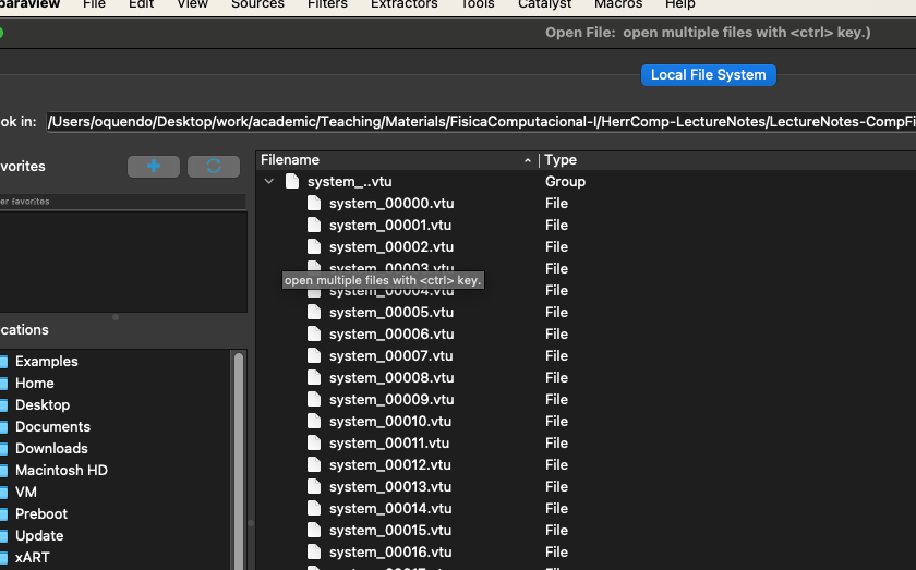
Now go and open Paraview, and then load the data using open and navigating the the folder where the data is (notice that paraview sees all data files as a series)
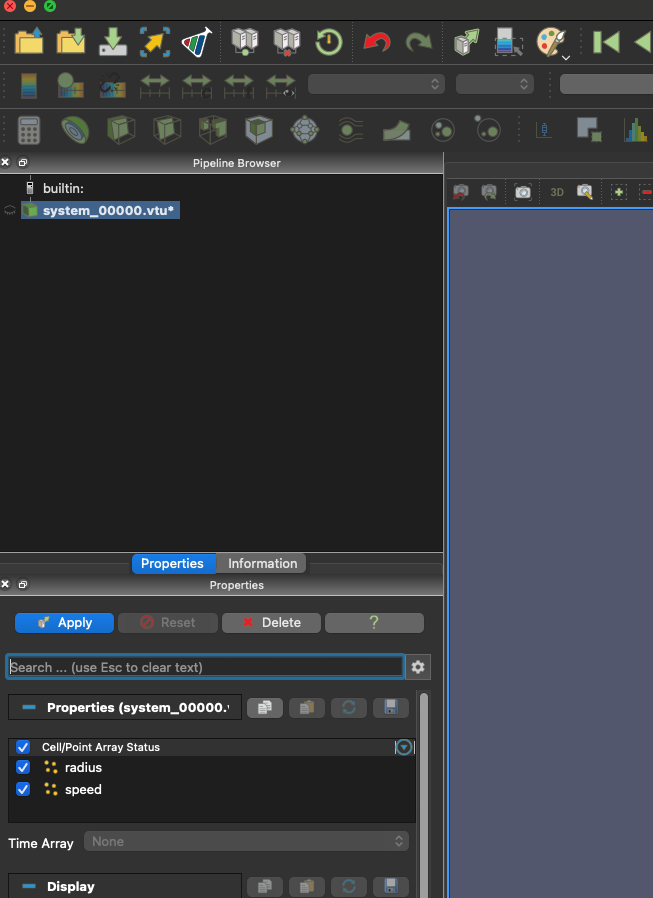
Then click on apply to actually load the series
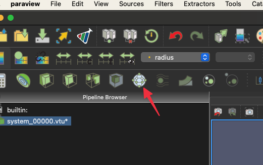
And, finally, apply some glyph (like spheres) to view the particles:
Then click play to see the actual animation. You can now use the powerful paraview filters and data analysis tools to understand better your system
Your exercise here is to adapt you md.py file to actually write the paraview data every NDISPLAY time steps, and then visualize the system using paraview.