Pseudo-random number generation

Pseudo-random number generation#

REFS:

Boudreau, Applied Computational Physics
Heath, Scientific Computing
Landau y Paez, Computational physics, problem solving with computers
Anagnostoupulos, A practical introduction to computational physics and scientific computing
Ward, Numerical Mathematicas and Computing

A random number routine is a mathematical rule allows to generate random numbers from a star point (seed) , numbers which hopefully are

not correlated
have a long period
are produced efficiently

Initial examples are the modulo generators,

(64)#\[\begin{equation} x_i = ax_{i-1} + c(\textrm{mod}\, m), \end{equation}\]

where the constants \(a, c, m\) should be chosen with care. For instance, \(m\) determines the period. A bad choice for those constant will lead to low period and large correlations. The generation of random numbers efficiently and with quality is an actual research topic, with huge implications from the field of random simulation of physical systems to the field of cryptography.

class random_naive:
    def __init__(self, seed):
        self.a = 1664525 # 1277
        self.c = 1013904223 # 0
        self.m = 2**32 # 2**17
        self.x = seed
        
    def r(self):
        self.x = (self.a*self.x + self.c)%self.m
        return self.x

rnum = random_naive(10)
for ii in range(10):
    print(rnum.r()/rnum.m)

23994349711574614
1856045601889491
6666164833586663
03803055686876178
048739948542788625
09891615808010101
654096252983436
8015652266331017
5949294364545494
15628248173743486

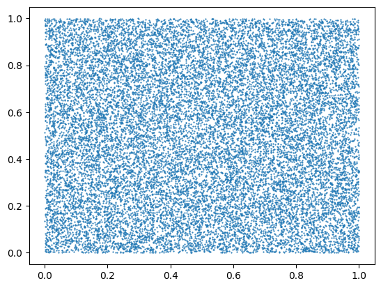
Unfortunately, this generator produces correlations

import numpy as np
import matplotlib.pyplot as plt
N = 20000
rnum = random_naive(1)
x = np.ones(N)
for ii in range(N):
    x[ii] = rnum.r()/rnum.m
fig, ax = plt.subplots()
ax.scatter(x[0:-1], x[1:], s=0.3)

<matplotlib.collections.PathCollection at 0x7f6ee07e4490>

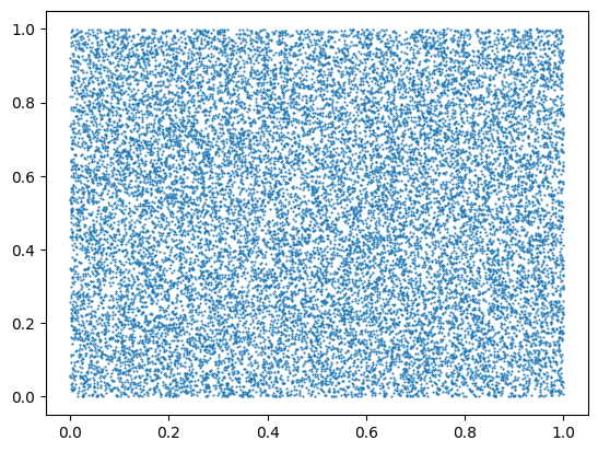
../_images/4559e1e10b6743ac56d828a0659d8ca00afe210bcbfc8fa04ce45df5e3a19340.png

Numpy random number generator#

Numpy has a powerfull and high quality random number generator. Some time ago they used the Mersenne Twister generator, which has a very large period and passes almost all tests successfully, but now they have moved to the PCG64 generator (see https://numpy.org/doc/stable/reference/random/generator.html and https://numpy.org/doc/stable/reference/random/bit_generators/pcg64.html#numpy.random.PCG64 )

The following is an example on how to use it (besides using a random seed)

import numpy as np
rng = np.random.default_rng(seed=42)
N = 20000
arr1 = rng.random((N,))
fig, ax = plt.subplots()
ax.scatter(arr1[0:-1], arr1[1:], s=0.3)

<matplotlib.collections.PathCollection at 0x7f6ee03f8e90>

../_images/c8e671c535fa9ace4d0bfdb3909a5c3a4720811e4fc2c145fc9070eead4a4ef3.png

Exercises:

[ ] Change the seed: do you notice any change?
[ ] Remove the seed and print the first ten numbers after running the cell several times: are they the same?

The numpy random generator produces numbers in \([0, 1)\), which can be transformed into other distributions. Furthermore, numpy also has some distributions already present (see https://numpy.org/doc/stable/reference/random/generator.html#distributions) . If your distribution is not on those already implemented, you will a method to generate variates, like the Rejection method, Ratio of uniforms, the inverse transform method, or many others.

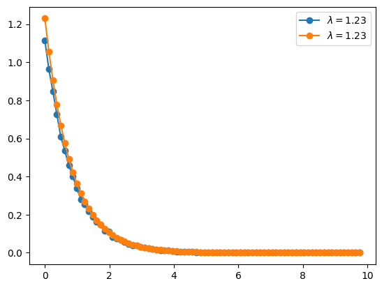
Inverse transform method#

In this case you want to invert the cumulative probability function. Let’s say that you have an exponential distribution, whose density is

(65)#\[\begin{equation} f(t) = \lambda e^{-\lambda t}, t > 0 \end{equation}\]

whose cumulative distribution is

(66)#\[\begin{equation} F(x) = \int_0^x f(t) dt = 1 - e^{-\lambda x}. \end{equation}\]

Now, the cumulative distribution is in the range \([0, 1]\). If we equate it to a uniform random number in the same interval, \(z = F(x)\), then we can invert this expression and obtain \(x = F^{-1}(z)\). For the exponential distribution we get

(67)#\[\begin{equation} x = -\frac{\ln (1-z)}{\lambda} \end{equation}\]

import numpy as np
import matplotlib.pyplot as plt

fig, ax = plt.subplots()
rng = np.random.default_rng(seed=21)
for LAMBDA in [1.23]:#, 2.34, 4.56]: 
    N = 40000
    z = rng.random((N,))
    x = -np.log(1-z)/LAMBDA
    hist, bin_edges = np.histogram(x, bins=80)
    # #ax.plot(x, 'o', ms=0.1)
    # ax.plot(bin_edges[:-1], hist, "-o", label=rf"$\lambda={LAMBDA}$")
    f = hist/(np.sum(hist)*(bin_edges[1:]-bin_edges[0:-1]))
    ax.plot(bin_edges[:-1], f, "-o", label=rf"$\lambda={LAMBDA}$")
    ax.plot(bin_edges[:-1], LAMBDA*np.exp(-LAMBDA*bin_edges[:-1]), "-o", label=rf"$\lambda={LAMBDA}$")
    
ax.legend()

<matplotlib.legend.Legend at 0x7f6ee03a2950>

../_images/f3bf42674b5b5a735acad4ee01f60c8587e30702a82dfa16a1753a6a169f38d4.png

Exercise:

[ ] Increase/decrease the number of samples
[ ] Increase/decrease the number of bins
[ ] Fit the data with an exponential function of the form \(ae^{-at}\). What is the \(a\) value? is what you expect?

Generating random samples in regions#

Let’s assume that you want to generate random samples uniformly distributed inside the ellipse \(x^2 + 4y^2 = 4\). To do so,

Generate random numbers \(-2 \le x \le 2\), and \(-1 \le y \le 1\), reject those outside the region.
In other cell, do the same but, to avoid wasting number, generate \(|y| \le \frac{1}{2}\sqrt{4-x^2}\).

Do you notice any difference?

# Solution to point 1
import numpy as np
import matplotlib.pyplot as plt
fig, ax = plt.subplots()

rng = np.random.default_rng(seed=21)
N = 10000
# YOUR CODE HERE
raise NotImplementedError()

---------------------------------------------------------------------------
NotImplementedError                       Traceback (most recent call last)
Cell In[6], line 9
      7 N = 10000
      8 # YOUR CODE HERE
----> 9 raise NotImplementedError()

NotImplementedError: 

../_images/9e13561b06f5d2c575e2e9d0ab28f3ca3efd7ae4d5738c0cd619a55149090489.png

%matplotlib inline
# Solution to point 2
import numpy as np
import matplotlib.pyplot as plt
fig, ax = plt.subplots()

rng = np.random.default_rng(seed=21)
N = 10000
# YOUR CODE HERE
raise NotImplementedError()

Exercises

[ ] Can you estimate the area from the previous computation (method 1)
[ ] Generate a random sample in the triangular region delimited by the x and y axis and the straight line \(y = 1-x\).
[ ] Generate a random uniform sample in the diamond figure with vertexes at \((1, 0), (0, 1), (-1, 0), (0, -1)\).
[ ] Generate a random uniform sample in a sphere, \(x^2 + y^2 + z^2 = R^2\). Count the fraction of numbers that are in the first octant.

Computing random integrals#

REF: Ward

Computing integrals using random numbers is easy and practical, specially for large dimensions. In the unit interval, one can compute

(68)#\[\begin{equation} \int_0^1 f(x) dx \simeq \frac{1}{n} \sum_{i=1}^n f(x_i), \end{equation}\]

so the integral is approximated as the average function value. For a general interval, one has

(69)#\[\begin{equation} \frac{1}{b-a}\int_a^b f(x) dx \simeq \frac{1}{n} \sum_{i=1}^n f(x_i), \end{equation}\]

or , in higher dimensions

(70)#\[\begin{equation} \frac{1}{8}\int_1^3\int_{-1}^1 \int_0^2 f(x, y, z) dxdydz \simeq \frac{1}{n} \sum_{i=1}^n f(x_i, y_i, z_i). \end{equation}\]

In general one has

(71)#\[\begin{equation} \int_A f \simeq (\text{measure of}\ A) \times (\text{average of}\ f\ \text{over}\ n\ \text{random points on}\ A) \end{equation}\]

Example#

Compute the following integral

(72)#\[\begin{equation} \iint_\limits{\Omega}\sin\sqrt{\ln(x+y+1)} dx dy, \end{equation}\]

where the integration region \(\Omega\) is the disk defined as \((x-1/2)^2 + (y-1/2)^2 \le 1/4\).

import numpy as np
import matplotlib.pyplot as plt
fig, ax = plt.subplots()
rng = np.random.default_rng(seed=21)

N = 10000
# YOUR CODE HERE
raise NotImplementedError()
# Expected value around 0.57

Example: Volume#

Now compute the volume of the following region

\begin{cases} &0 \le x\le 1,\ 0 \le y\le 1, \ 0 \le z\le 1, \ &x^2 + \sin y\le z, \ &x -z + e^y \le 1. \end{cases} The expected value is around 0.14

import numpy as np
import matplotlib.pyplot as plt
rng = np.random.default_rng(seed=21)

N = 10000
# YOUR CODE HERE
raise NotImplementedError()
print(VOLUME)

Exercises

[ ] (Ward) Compute

(73)#\[\begin{equation} \int_0^2\int_3^6\int_{-1}^1 (y x^2 + z\log y + e^x) dx dy dz \end{equation}\]
[ ] Compute the area under the curve \(y = e^{-(x+1)^2}\)
(Boudreau, 7.8.7) Estimate the volume of an hypersphere in 10 dimensions. The convergence rate is equal to \(C/\sqrt M\), where \(M\) is the total number of samples. Estimate the value of \(C\). Is it the same for 20 dimensions?

# YOUR CODE HERE
raise NotImplementedError()

A first simulation: the random walk#

The so-called MonteCarlo methods are computational methods that use random numbers to perform computations or simulations. Applications are extense, from traffic simulations, to atomic systems, to pedestrian crowds, to probabilistic computations, to neutron scattering in nuclear shielding, to materials design, and so on.

Up to now, we have used random numbers to perform some computations. Now let’s simulate a very simple process ,as an introduction to the field of MonteCarlo: the random walk, which is an example of random process.

We will define a grid, and our walker will chose the next position at random. We are interested in computing the mean squared distance as function of time, which is related with a diffusion process.

import numpy as np

import matplotlib.pyplot as plt
def random_walk(seed, nsteps, ax):
    rng = np.random.default_rng(seed=seed)
    x = np.zeros(nsteps)
    y = np.zeros(nsteps)
    # YOUR CODE HERE
    raise NotImplementedError()
    ax.plot(x, y)
    
NSTEPS = 10000
fig, ax = plt.subplots()
random_walk(10, NSTEPS, ax)
random_walk(2, NSTEPS, ax)
random_walk(7, NSTEPS, ax)

Exercise

[ ] Compute the mean squared distance as a function of time
[ ] Simulate a 3D random walk
[ ] Simulate a loaded dice with the following probabilities. Perform 10000 throws and plot the final distribution. | Outcome | 1 | 2| 3| 4| 5| 6| |-|-|-|-|-|-|-| | Probability | 0.2 | 0.14 | 0.22 | 0.16 | 0.17 | 0.11|