1D Arrays for 2D Matrices#
Representing a matrix#
A matrix is a 2d array of objects (numbers in our case) with m rows and n columns, with a total of \(S=m\times n\) elements. See
Rotations and scaling: https://www.cs.usfca.edu/~galles/visualization/RotateScale2D.html
Matrices are ubiquitous in physics and mathematics, and their manipulation are the core of a large proportion of computational and numerical problems. Efficient matrix manipulation and characteristic computing must be very performant and scalable. That is why, normally, you should always use a specialized library to solve typical problems like \(Ax=b\), or to compute eigen values and eigen vectors, determinants and so on, but , outside the realm of linear algebra matrices are heavily used so you need to know how to represent and manipulate them.
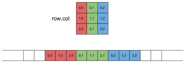
Normally, a matrix will be indexed as \(A_{ij}\), with the first index representing the row and the second one the column. You must be aware that sometimes the indexes start at 1 and sometimes at 0. In c++ your indexes start at 0. Even though the matrix is a 2D array, it will be represented as an array of arrays in memory given that the ram memory is linear, as shown in https://en.wikipedia.org/wiki/Matrix_representation?useskin=vector and https://eli.thegreenplace.net/2015/memory-layout-of-multi-dimensional-arrays . For 2D arrays, you have basically two options:
row-major
column-major
For instance, the following code shows the row-major ordering in c/c++, using old/primitive arrays:
    // REF: https://scicomp.stackexchange.com/questions/37264/how-much-space-store-a-matrix-of-numbers
    #include <iostream>

    int main(int argc, char **argv) {
      const int N = 4;
      int m[N][N] = {0}; //4 by4 matrix with all zeros (default value for ints) allocated on the stack
      for (unsigned int i = 0; i < N; ++i) {
        for (unsigned int j = 0; j < N; ++j) {
          std::cout << &m[i][j] << "\t";
        }
        std::cout << "\n";
      }
      return 0;
    }
| 0x16b2cadb8 | 0x16b2cadbc | 0x16b2cadc0 | 0x16b2cadc4 |
| 0x16b2cadc8 | 0x16b2cadcc | 0x16b2cadd0 | 0x16b2cadd4 |
| 0x16b2cadd8 | 0x16b2caddc | 0x16b2cade0 | 0x16b2cade4 |
| 0x16b2cade8 | 0x16b2cadec | 0x16b2cadf0 | 0x16b2cadf4 |
Run this on your system. Do you get the same addresses? are they continuous?
Defining matrices from primitives in C++#
In C++, matrices there could be defined in several ways :
Primitive array in the stack (contiguous but limited in size)
    double A[M][N];
    ...
    A[2][0] = 59.323;
Primitive dynamic array (not guaranteed to be contiguous in memory):
    double **A;
    A = new double *[M];
    for (int ii = 0; ii < M; ++ii) {
      A[ii] = new double [N];
    }
    //...
    for (int ii = 0; ii < M; ++ii) {
      delete A[ii];
    }
    delete [] A;
    A = nullptr;
A array of arrays : In the stack, limited size
std::array<std::array<double, N>, M> A;
A vector of vectors : not guaranteed to be contiguous in memory
    std::vector<std::vector<double>> A;
    A.resize(M);
    for (int ii = 0; ii < M; ++ii) {
      A[ii].resize(N);
    }
All the previous are fine if you don’t care about memory size or contiguous
memory. But in scientific computing, applied to physics, we need to create
performant data structures. For that reason we need to just ask for block of memory
of size M*N and then view it as a 2D array using index tricks.
1D and 2D view#
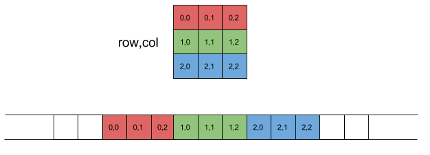
Being efficient when accessing memory is key to get a good performance. How are 2D arrays stored in memory? Assume that you have the following 2D array (data inside each cell correspond to indexes)

As you can see, in the 1d array in memory, the first element (1d index 0) has the coordinates (0, 0), the second element (1d index 1) corresponds to (0, 1), and so on. The sixth 1d element, with 1d index 5, has 2D coordinates (1, 2). Can you devise a rule to relate the 1d and the 2d indexes?
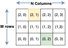
We start from a 2D array as

In a row-major language, like c++, it will be organized as a 1D array, row after row. We want to go through it in the same order, so we want to get a mapping like:

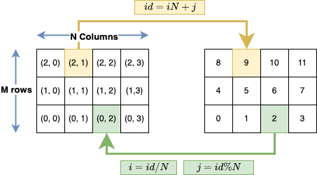
This will allow having an MxN size 1d array, but interpreting it as a 2D array, using the following mapping
while , from 1D to 2D

In other words, to reference an element [i][j], you just use [i*N + j], where N is the total number of columns.
Practical Example: transposing a matrix#
In this example, you will implement a matrix transpose but using 1d arrays. We will use two matrices, A and B, whose dimensions will be read from the command line, and will be modelled using 1d arrays. We will initialize A as
Since \(B = A^T\), if A is of size MxN, then B is of size NxM (although their total size is the same, M*N). Complete the following code:
#include <iostream>
#include <vector>
#include <string>

void fill_matrix(std::vector<double> & data, int m, int n);
void print_matrix(const std::vector<double> & data, int m, int n);
void transpose_matrix(const std::vector<double> & indata, int m, int n,
                      std::vector<double> & outdata);

int main(int argc, char **argv)
{
  const int M = std::stoi(argv[1]);
  const int N = std::stoi(argv[2]);

  std::vector<double> array2d(M*N, 0.0);

  fill_matrix(array2d, M, N);
  print_matrix(array2d, M, N);

  std::vector<double> array2d_T(M*N, 0.0);
  transpose_matrix(array2d, M, N, array2d_T);
  print_matrix(array2d_T, N, M);

  return 0;
}

void fill_matrix(std::vector<double> & data, int m, int n)
{
  for (int ii = 0; ii < m; ++ii) {
    for (int jj = 0; jj < n; ++jj) {
      data[ii*n + jj] = ii*n+jj; // A_(i, j) = i*n + j = id
    }
  }
}

void print_matrix(const std::vector<double> & data, int m, int n)
{
  for (int ii = 0; ii < m; ++ii) {
    for (int jj = 0; jj < n; ++jj) {
      std::cout << data[ii*n + jj] << " ";
    }
    std::cout << "\n";
  }
  std::cout << "\n";
}

void transpose_matrix(const std::vector<double> & datain, int m, int n,
                      std::vector<double> & dataout)
{
  // TODO
//=== BEGIN MARK SCHEME ===
  for (int ii = 0; ii < m; ++ii) {
    for (int jj = 0; jj < n; ++jj) {
      dataout[ii*m + jj] = datain[ii*n + jj]; // Error here
    }
  }
//=== END MARK SCHEME ===
}
Exercises#
For the following exercises, and unless stated otherwise, the size of the matrices must be read from the command line and also the matrices must be filled randomly using a uniform random distribution in [-1, 1]. Also, the random seed must be read from the command line. Furthermore, the solutions must be modularized as follows:
matrix_utils.h: All the functions declarations and includes must come here. Each exercise implies one or more new declarations in this file.matrix_utils.cpp: All the functions implementations come here.main_XXXX.cpp: Each exercise will be solved in a main file where the necessary functions are called. The filename will change (theXXXXpart).
Then you will need to compile as
g++ -std=c++17 -fsanitize=undefined,address,leak matrix_utils.cpp matrix_XXXX.cpp
Here is a basic example is show for the three files. Remember: the files
matrix_utils.cpp/h will grow with new functions implemented there. The file
main_XXXX.cpp will have a different name for each exercise and call different
functions.
matrix_utils.h: Declarations.
#pragma once
#include <iostream>
#include <vector>
#include <cassert>
#include <random>
void print_matrix(const std::vector<double> & M, int nrows, int ncols);
void fill_matrix_random(std::vector<double> & M, const int nrows, const int ncols, const int seed);
matrix_utils.cpp: Implementations
#include "matrix.h"
void print_matrix(const std::vector<double> & M, int nrows, int ncols){
    std::cout.setf(std::ios::scientific);
    std::cout.precision(15);

    for (int ii = 0; ii < nrows; ++ii) {
        for (int jj = 0; jj < ncols; ++jj) {
            std::cout << M[ii*ncols + jj] << " "; // (ii, jj) = ii*NCOLS + jj
        }
        std::cout << "\n";
    }
    std::cout << "\n";
}
void fill_matrix_random(std::vector<double> & M, const int nrows, const int ncols, const int seed){
    std::mt19937 gen(seed);
    std::uniform_real_distribution<> dis(-1, 1);
    for (int ii = 0; ii < nrows; ii++){
        for (int jj = 0; jj < ncols; jj++){
            M[ii*ncols + jj] = dis(gen);
        }
    }

}
main_example.cpp: Simple example
#include "matrix.h"

int main(int argc, char **argv) {
    // read size of matrix
    if (argc != 3) {
        std::cerr << "Error. Usage:\n"
                  << argv[0] << " M N \n"
                  << "M : Rows\n"
                  << "N : Columns\n";
        return 1;
    }
    const int M = std::stoi(argv[1]);
    const int N = std::stoi(argv[2]);

    // create matrix A
    std::vector<double> A(M*N);

    // fill matrix randomly
    fill_matrix_random(A, M, N, 0); // 0 == seed

    // print matrix
    print_matrix(A, M, N);

    return 0;
}
Trace of a matrix#
Compute the trace of a random matrix using 1D indexing.
Hilbert matrix#
Create a function to compute the trace of that matrix. Fill the matrix as the Hilbert Matrix, \(A_{ij} = 1/(i +j +1)\)
Implement matrix-matrix multiplication#
A function must received the two input matrices and an output matrix and write there the result.
\(A \times A^t\)#
Implement a function to compute the matrix multiplication of matrix with its transpose.
\(A^p\)#
Implement a function to compute the power of a matrix performing successive multiplications.
Idempotent matrix#
Implement a function that receives a matrix and a power and checks if it is idempotent under some precision, that is, if \(|A^p - A| < \epsilon\), where the norm is evaluated checking the inequality element-by-element.
Checking inverse#
Implement a function that receives two matrices and check if they are inverse of each other, that is , if \(|AB - I| < \epsilon\) and \(|BA - I| < \epsilon\), where the check is done on each element.
Matrix commute#
Write a function that receives two matrices and checks if they commute under a given precision, that is , \(|AB - BA| < \epsilon\).
Orthogonal matrix#
Implement a function that receives a matrix and checks if it is orthogonal, that is, if \(|A A^T - I| < \epsilon\), where the norm is evaluated checking the inequality element-by-element.
Matrix of complex numbers#
Implement a function that receives a matrix OF COMPLEX NUMBERS and checks if it is hermitian,
that is, if \(|A A^\dagger - I| < \epsilon\), where the norm is evaluated checking the
inequality element-by-element. Use the <complex> header. \(A^\dagger\) means the
transpose conjugate.
Pauli matrix#
Write a function that receives three components of a vectors and saves the corresponding Pauli-vector-matrix: https://en.wikipedia.org/wiki/Pauli_matrices#Pauli_vector
Complex matmul and Pauli matrices#
Extend your multiplication routine to use complex numbers and check the Pauli matrix commutation relations: https://en.wikipedia.org/wiki/Pauli_matrices#(Anti-)Commutation_relations
Vandermonde matrix#
Write a routine to fill a matrix as a Vandermonde matrix, https://en.wikipedia.org/wiki/Vandermonde_matrix , and then compute and print its trace Read the number of rows from the command line
Matrix polynomial#
Implement a function that receives a matrix and an array representing the coefficients of a polynomial, \(a_0, a_1, \ldots, a_n\), and evaluates that polynomial on the given matrix, \(a_0 I + a_1 A + a_2 A^2 + \ldots + a_n A^n\), and stores the result in an output matrix.
Matmul time performance#
Matrix multiplication time: Explore how the total multiplication time grows with the matrix size. The following code is a template. You should read it and understand it carefully. Implement what is needed.
        #include <iostream>
        #include <chrono>
        #include <random>
        #include <cmath>
        #include <cstdlib>
        #include <vector>
        #include <algorithm>

        void multiply(const std::vector<double> & m1, const std::vector<double> & m2, std::vector<double> & m3);

        int main(int argc, char **argv) {
          // read parameters
          const int N = std::atoi(argv[1]);
          const int SEED = std::atoi(argv[2]);

          // data structs
          std::vector<double> A(N*N, 0.0), B(N*N, 0.0), C(N*N, 0.0);

          // fill matrices A and B, using random numbers betwwen 0 and 1
          std::mt19937 gen(SEED);
          std::uniform_real_distribution<> dist(0.,1.);
          // lambda function: a local function that captures [] something, receives something (), and return something {}
          // See: https://www.learncpp.com/cpp-tutorial/introduction-to-lambdas-anonymous-functions/
          std::generate(A.begin(), A.end(), [&gen, &dist](){ return dist(gen); }); // uses a lambda function
          std::generate(B.begin(), B.end(), [&gen, &dist](){ return dist(gen); }); // uses a lambda function

          // multiply the matrices A and B and save the result into C. Measure time
          auto start = std::chrono::high_resolution_clock::now();
          multiply(A, B, C);
          auto stop = std::chrono::high_resolution_clock::now();

          // use the matrix to avoid the compiler removing it
          std::cout << C[N/2] << std::endl;

          // print time
          auto elapsed = std::chrono::duration<double>(stop - start);
          std::cout << elapsed.count() << "\n";

          return 0;
        }

        // implementations
        void multiply(const std::vector<double> & m1, const std::vector<double> & m2, std::vector<double> & m3)
        {
          const int N = std::sqrt(m1.size()); // assumes square matrices
          delete this line and implement the matrix multiplication here
        }
When run as
./a.out 64 10
you should get something like
Value |
|
|---|---|
1 |
14.6676 |
2 |
0.002486 |
Plot, in log-log scale, the time as a function of the matriz size \(N\) in the range \(N \in \{4, 8, 16, 32, 64, 128, 256, 512, 1024\}\). Normalize all times by the time at \(N = 4\).


