Efficient Python arrays : Numpy#
REFS:
A primer of Scientific Programming with Python
https://betterprogramming.pub/numpy-illustrated-the-visual-guide-to-numpy-3b1d4976de1d
The numerical python package, numpy, allows for easy and efficient manipulation of vectorial data. In this context, it is important to remark some of the so-called vectorial computation. Let’s give an example. Imagine a two dimensional vector \(a\). How would you represent it using python? You coul use either a list, a tuple, etc:
a1 = [x, y]
a2 = (x, y)
Of course, it can be generalized to more dimensions:
a1 = [x, y, z, w]
a2 = [0.0, -0.9, 1, -3, 9, ... , 90]
Managing vectors by using these typical python constructs is very good from a general programmer point of view, but it has its costs. For example, iterating over a lits by means of a for loop could be very slow. Actually, for typical problemas of computational mathematics and physics, only homogeneous storage structs with fast access are needed, like the arrays of languages like c++, fortran, etc. Arrays might be more limited than general lists, but could vastly outperform lists and tuples for vectorial computations. The numpy package provides array like structs to perform fast mathematical operations on numerical data.
Furthermore, vectorial operations are natural on numpy arrays. But what is a vectorial operation? Let’s assume we have a vector \(v\) of \(n\)-components. What would be the meaning of something like
u = sin(v)
? in the context of vectorial computing, it would mean to apply the function sin to every component of the vector v, therefore \(u_i = \sin(v_i)\). In general, given a function \(f\), the expression \(u = f(v)\) means \(u_i = f(v_i)\). Numpy allows for this kind of computing. What would be the meaning of
u = v^2*cos(v)*e^v + 2?

See: https://betterprogramming.pub/numpy-illustrated-the-visual-guide-to-numpy-3b1d4976de1d
Basic numpy#
Try the following code snippet:
import numpy as np
a = np.array([0, 1.0, '3', 5])
print (a)
a.dtype
['0' '1.0' '3' '5']
dtype('<U32')
This means: we are importing the numpy package with the name np. Then, we create an numpy array by using the np.array function from a list of values, and assign the result to the variable a. What is a? use a? . The array a has several attributes which you can use later, like the shape and type of the internal data.
Let’s now compare the efficiency of a list versus a numpy array, by means of the %timeit magic function of ipython:
L = range(10000)
%timeit [i**2 for i in L]
414 μs ± 11.9 μs per loop (mean ± std. dev. of 7 runs, 1,000 loops each)
a = np.arange(10000)
%timeit a**2
2.54 μs ± 15.5 ns per loop (mean ± std. dev. of 7 runs, 100,000 loops each)
You can extract some info like the shape and the dimension as
a.ndim
1
a.shape
(10000,)
a.dtype
dtype('int64')
Alternative ways to create arrays#
a = np.arange(10)
b = np.arange(1, 9, 2)
The function linspace is very useful. It allows to create a uniform partition on a given interval for a given number of points. For example, to create an array of 100 points uniformly on the interval [2, 3], you can use
a = np.linspace(2, 3, 100)
print a
  Cell In[7], line 2
    print a
    ^
SyntaxError: Missing parentheses in call to 'print'. Did you mean print(...)?
Check the documentation.
You can also create several other types of useful arrays like
a = np.ones((3, 4)) # shape is a tuple
print a
a = np.random.rand(4)
print a
[ 0.900158 0.23643884 0.70674432 0.53132537]

Ref: https://betterprogramming.pub/numpy-illustrated-the-visual-guide-to-numpy-3b1d4976de1d
# Truncation errors
data = np.arange(0.5, 0.8, 0.1)
print(f"{data = }") # should not include 0.8
data = array([0.5, 0.6, 0.7, 0.8])
# Solution: dont use floats, use integers
data = 0.1*np.arange(5, 8)
print(f"{data = }")
data = 0.5 + 0.1*np.arange(0, 3)
print(f"{data = }")
data = array([0.5, 0.6, 0.7])
data = array([0.5, 0.6, 0.7])
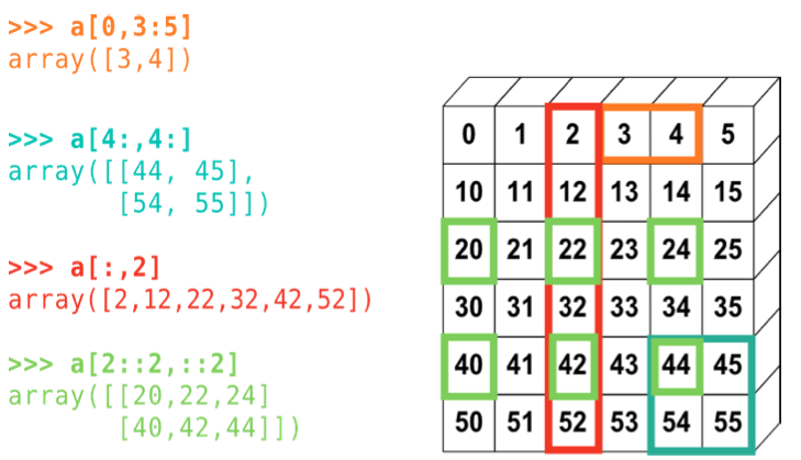
Indexing and slicing#
Numpy allows for powerfull and efficient access to internal members of arrays
from IPython.core.display import Image
Image(filename='slicing.png')
Copies and Views#
A slicing operation creates a view of the original array, not a copy (in contrast, an slice of a list creates a new list). A modification of a view, modifies the original array:
a = np.arange(10)
print (a)
b = a[::2]
print (b)
b[0] = 12
print (b)
print (a)
[0 1 2 3 4 5 6 7 8 9]
[0 2 4 6 8]
[12  2  4  6  8]
[12  1  2  3  4  5  6  7  8  9]
But, if you really need a copy, you can use the .copy method:
a = np.arange(10)
print (a)
c = a[::2].copy()
c[0] = 12
print (a)
print (c)
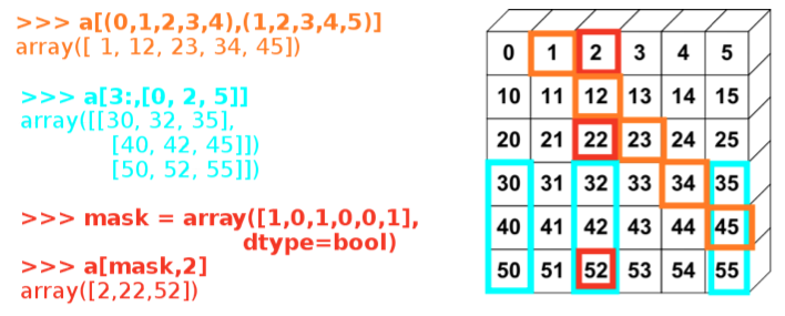
Fancy indexing (masked arrays)#
Using arrays to mask indexes is an useful way to manipulate arrays. Numpy provides this functionality. Note: Fancy indexing creates copies, not views.
Boolean masks#
np.random.seed(3)
a = np.random.random_integers(0, 20, 15)
print (a)
print (a % 3 == 0)
mask = (a % 3 == 0)
print ("Mask = ", mask)
[10  3  8  0 19 10 11  9 10  6  0 20 12  7 14]
[False  True False  True False False False  True False  True  True False
  True False False]
Mask =  [False  True False  True False False False  True False  True  True False
  True False False]
extract_from_a = a[mask]
print (extract_from_a)
[ 3 0 9 6 0 12]
print (a)
a[a%3 == 0] = -1
print (a)
[10  3  8  0 19 10 11  9 10  6  0 20 12  7 14]
[10 -1  8 -1 19 10 11 -1 10 -1 -1 20 -1  7 14]

Ref: https://betterprogramming.pub/numpy-illustrated-the-visual-guide-to-numpy-3b1d4976de1d
Indexing with integers#
a = np.arange(0, 100, 10)
print a
a[[2, 3, 2, 4, 2]]
[ 0 10 20 30 40 50 60 70 80 90]
array([20, 30, 20, 40, 20])
a[[9, 7]] = -100
print a
[ 0 10 20 30 40 50 60 -100 80 -100]
Image(filename='fancy_indexing.png')
Numerical operations (or vector computing)#
As stated at the beginning, numpy arrays are well suited for the so called numerical computing. In this section we will see some examples to get familiar with this kind of operations.
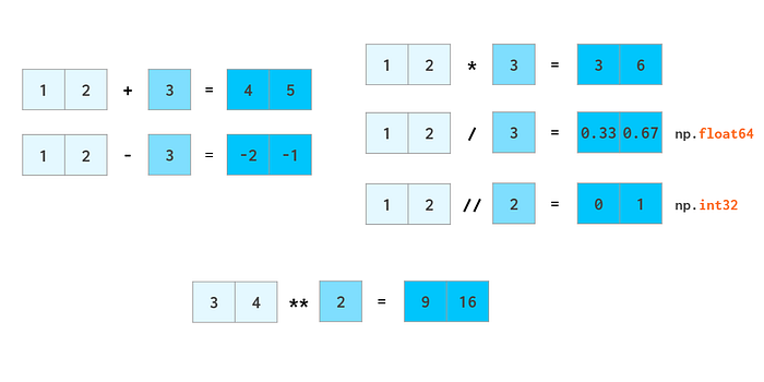 From: https://betterprogramming.pub/numpy-illustrated-the-visual-guide-to-numpy-3b1d4976de1d
a = np.array([1, 2, 3, 4])
print (a)
print (a + 1)
print (2*a)
[1 2 3 4]
[2 3 4 5]
[2 4 6 8]
b = np.ones(4) + 1
print (b)
b-a
[ 2. 2. 2. 2.]
array([ 1., 0., -1., -2.])
j = np.arange(5)
2**(j + 1) - j
Performance comparison:
a = np.arange(10000)
%timeit a + 1
10000 loops, best of 3: 20.2 µs per loop
l = range(10000)
%timeit [i+1 for i in l]
1000 loops, best of 3: 882 µs per loop
Take into account that array multiplication should be done through function np.dot
You can use a lot of internal functions (https://numpy.org/doc/stable/reference/routines.math.html) and random generators (https://numpy.org/doc/stable/reference/random/index.html)
2D Arrays#

REF: https://betterprogramming.pub/numpy-illustrated-the-visual-guide-to-numpy-3b1d4976de1d
Axis#

REF: https://betterprogramming.pub/numpy-illustrated-the-visual-guide-to-numpy-3b1d4976de1d
Matrix aggregation#
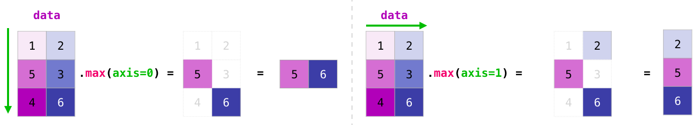
REF: https://jalammar.github.io/visual-numpy/


Exercises#
Reading a file#
Create a Reading a two column file: Make a program who reads a two column file and stores the first column in a list called x and the second one in a list called y. Then convert the list to arrays and plot them. Test it with some example file.
# YOUR CODE HERE
raise NotImplementedError()
Reading file with comments#
Extend the previous exercise to be able to read a data file with comments. The comment chracter is supposed to be #. Every line starting with # should be ignored. Test.
# YOUR CODE HERE
raise NotImplementedError()
Using loadtxt#
Improve exercise 1 and 2 by using the numpy.loadtxt() function. You should rerad the documentation. Test and compare.
# YOUR CODE HERE
raise NotImplementedError()
Printing with comments#
Write a program which prints tabulated data for a given function, but also printing some comments on it using the # character. Use the previous program to make sure you can read back the data.
# YOUR CODE HERE
raise NotImplementedError()
Kinematics from file#
Assume that you are given a file which has printed the values \(a_0, a_1, \ldots, a_k\) for the acceleration of a given system at specified intervals of size \(\Delta t\), that is, \(t_k = k\Delta t\). Your task is to read those values and to compute the velocity of the system at some time \(t\). To do that remember that the acceleration can be given as \(a(t) = v'(t)\). Therefore, to find \(v\), you must integrate the acceleration as
If \(a(t)\) is only known at discrete points, as in this case, you have to approximate the integral. You can use the trapezoidal rule to get
Assume that \(v(0) = 0\). Your program should: Read the values for \(a\) from the array. Then, compute the values for velocity and finally plot the acceleration and the velocity as a function of time. Good test cases for this problem are null values for the acceleration, and constant values for the acceleration, whose theoretical solution you already know. The \(\Delta t\) value should be specified at the command line (use the sys module to read command line arguments).
# YOUR CODE HERE
raise NotImplementedError()
3D matrix example: Image#
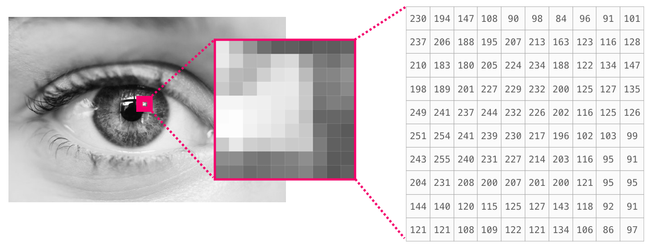
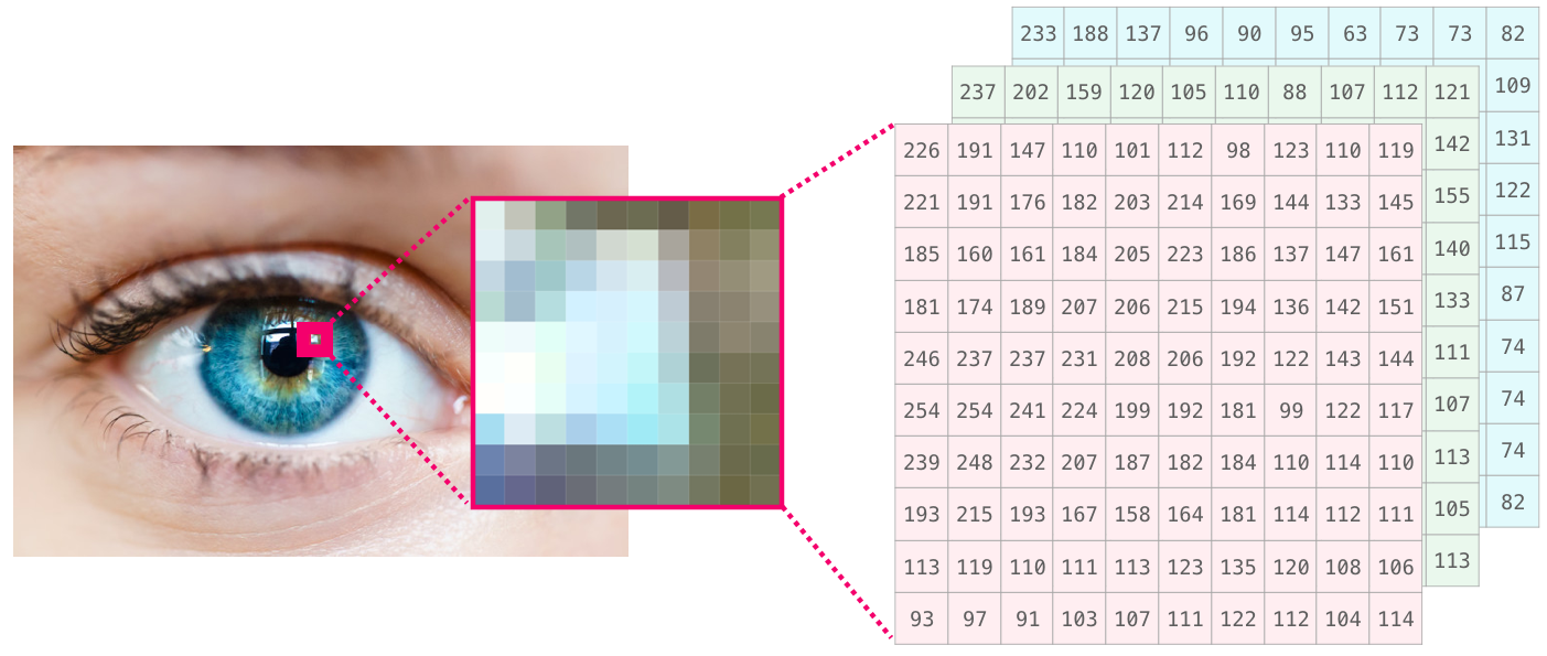
REF: https://jalammar.github.io/visual-numpy/
Image tutorial example#
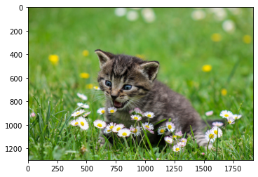
We will use the following kitty image: https://files.realpython.com/media/kitty.90952ca484f1.jpg from https://realpython.com/numpy-tutorial/ . The local name will be just kitty.jpg .

import numpy as np
import matplotlib.image as mpimg

img = mpimg.imread("kitty.jpg")
print(type(img))
print(img.shape)
<class 'numpy.ndarray'>
(1299, 1920, 3)
import matplotlib.pyplot as plt
imgplot = plt.imshow(img)
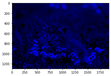
# Now remove the red and green channels
output = img.copy()  # The original image is read-only!
output[:, :, :2] = 0
mpimg.imsave("kitty-blue.jpg", output)
img_blue = mpimg.imread("kitty-blue.jpg")
imgplot_blue = plt.imshow(img_blue)
# Now make it only green
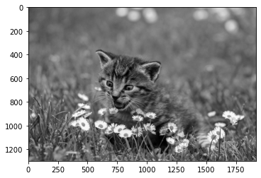
# Now let's make it gray-scale
# This means averaging all the channels
averages = img.mean(axis=2)  # Take the average of each R, G, and B
mpimg.imsave("kitty-bad-gray.jpg", averages, cmap="gray")
img_gray = mpimg.imread("kitty-bad-gray.jpg")
imgplot_gray = plt.imshow(img_gray)
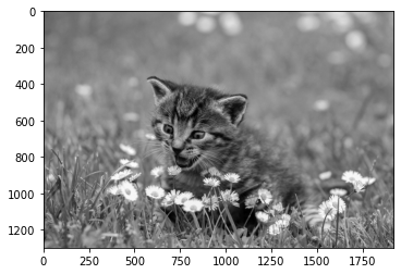
# Now improve it by using the luminosity method:
# Differente weigths for each channel
weights = np.array([0.3, 0.59, 0.11])
grayscale = img @ weights # dot product
mpimg.imsave("kitty-good-gray.jpg", grayscale, cmap="gray")
img_gray = mpimg.imread("kitty-good-gray.jpg")
imgplot_gray = plt.imshow(img_gray)
#!pip3 install --user scikit-image
!conda install -y scikit-image
Collecting package metadata (current_repodata.json): done
Solving environment: done

## Package Plan ##

  environment location: /home/oquendo/miniconda3

  added / updated specs:
    - scikit-image


The following packages will be downloaded:

    package                    |            build
    ---------------------------|-----------------
    cytoolz-0.11.0             |   py38h96a0964_3         344 KB  conda-forge
    dask-core-2021.8.1         |     pyhd8ed1ab_0         764 KB  conda-forge
    enum34-1.1.10              |   py38h32f6830_2           4 KB  conda-forge
    fsspec-2021.7.0            |     pyhd8ed1ab_0          81 KB  conda-forge
    imagecodecs-lite-2019.12.3 |   py38hc7193ba_3         171 KB  conda-forge
    locket-0.2.0               |             py_2           6 KB  conda-forge
    networkx-2.5.1             |     pyhd8ed1ab_0         1.2 MB  conda-forge
    openssl-1.1.1k             |       h0d85af4_1         1.9 MB  conda-forge
    partd-1.2.0                |     pyhd8ed1ab_0          18 KB  conda-forge
    pooch-1.4.0                |     pyhd8ed1ab_0          41 KB  conda-forge
    pywavelets-1.1.1           |   py38hc7193ba_3         4.3 MB  conda-forge
    scikit-image-0.18.2        |   py38h1f261ad_0        11.0 MB  conda-forge
    tifffile-2019.7.26.2       |           py38_0         219 KB  conda-forge
    ------------------------------------------------------------
                                           Total:        20.0 MB

The following NEW packages will be INSTALLED:

  cytoolz            conda-forge/osx-64::cytoolz-0.11.0-py38h96a0964_3
  dask-core          conda-forge/noarch::dask-core-2021.8.1-pyhd8ed1ab_0
  enum34             conda-forge/osx-64::enum34-1.1.10-py38h32f6830_2
  fsspec             conda-forge/noarch::fsspec-2021.7.0-pyhd8ed1ab_0
  imagecodecs-lite   conda-forge/osx-64::imagecodecs-lite-2019.12.3-py38hc7193ba_3
  imageio            conda-forge/noarch::imageio-2.9.0-py_0
  locket             conda-forge/noarch::locket-0.2.0-py_2
  networkx           conda-forge/noarch::networkx-2.5.1-pyhd8ed1ab_0
  partd              conda-forge/noarch::partd-1.2.0-pyhd8ed1ab_0
  pooch              conda-forge/noarch::pooch-1.4.0-pyhd8ed1ab_0
  pywavelets         conda-forge/osx-64::pywavelets-1.1.1-py38hc7193ba_3
  scikit-image       conda-forge/osx-64::scikit-image-0.18.2-py38h1f261ad_0
  tifffile           conda-forge/osx-64::tifffile-2019.7.26.2-py38_0
  toolz              conda-forge/noarch::toolz-0.11.1-py_0

The following packages will be UPDATED:

  openssl                                 1.1.1k-h0d85af4_0 --> 1.1.1k-h0d85af4_1


Downloading and Extracting Packages
fsspec-2021.7.0      | 81 KB     | ##################################### | 100%
scikit-image-0.18.2  | 11.0 MB   | ##################################### | 100%
openssl-1.1.1k       | 1.9 MB    | ##################################### | 100%
dask-core-2021.8.1   | 764 KB    | ##################################### | 100%
cytoolz-0.11.0       | 344 KB    | ##################################### | 100%
enum34-1.1.10        | 4 KB      | ##################################### | 100%
networkx-2.5.1       | 1.2 MB    | ##################################### | 100%
partd-1.2.0          | 18 KB     | ##################################### | 100%
tifffile-2019.7.26.2 | 219 KB    | ##################################### | 100%
pooch-1.4.0          | 41 KB     | ##################################### | 100%
pywavelets-1.1.1     | 4.3 MB    | ##################################### | 100%
locket-0.2.0         | 6 KB      | ##################################### | 100%
imagecodecs-lite-201 | 171 KB    | ##################################### | 100%
Preparing transaction: done
Verifying transaction: done
Executing transaction: done
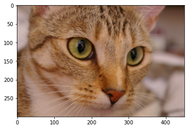
from skimage import data
cat = data.chelsea()
type(cat)
cat.shape
(300, 451, 3)
plt.imshow(cat)
<matplotlib.image.AxesImage at 0x13f084940>
Exercise#
Obtain the following image (zoom on 1/4 to 3/4 on each axis):
